Function to choose optimal forecast model for quarterly data
QuarterModelPicker.RdFunction to choose optimal forecast model for quarterly data
QuarterModelPicker(data, Outcome, DateVar, H.Horizon = 12)
Arguments
| data | A quarterly tsibble. |
|---|---|
| Outcome | A valid variable name for the Outcome to be modelled in in `data`. |
| DateVar | A valid variable name for the time index in `data`. |
| H.Horizon | An integer for the forecast horizon/test subset of `data`. |
Value
A list containing:
Accuracy.Table: accuracy for the forecast horizon against the test sample.
test: the test set
train: the training set
Model.Fits: the model fits
Model.Forecasts: the forecasts
Min.Model: the minimum model by MAE
Min.Report: the minimum model report
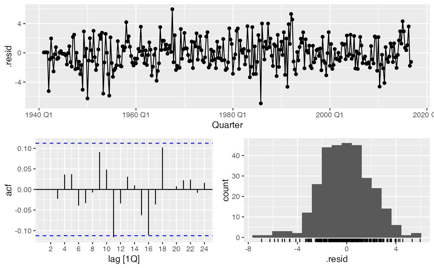
Min.Res.Plot: the gg_tsdisplay for the minimum model
Min.Forecast.Plot: a plot of the minimum forecast by MAE
Examples
#> Warning: Current temporal ordering may yield unexpected results. #> ℹ Suggest to sort by ``, `Quarter` first.#>#> Warning: 1 error encountered for K = 3 #> [1] K must be not be greater than period/2#> Warning: 1 error encountered for NNET3 #> [1] K must be not be greater than period/2#> Warning: Current temporal ordering may yield unexpected results. #> ℹ Suggest to sort by ``, `Quarter` first.#> Warning: Current temporal ordering may yield unexpected results. #> ℹ Suggest to sort by ``, `Quarter` first.#> Warning: Current temporal ordering may yield unexpected results. #> ℹ Suggest to sort by ``, `Quarter` first.#> Series: TX #> Model: ARIMA(1,0,2)(0,1,1)[4] w/ drift #> #> Coefficients: #> ar1 ma1 ma2 sma1 constant #> 0.6870 -0.4961 0.0189 -0.9538 0.0085 #> s.e. 0.1846 0.1938 0.0768 0.0217 0.0041 #> #> sigma^2 estimated as 4.181: log likelihood=-642.42 #> AIC=1296.84 AICc=1297.12 BIC=1319.06#> $test #> # A tsibble: 12 x 5 [1Q] #> Quarter TX TN PR SN #> <qtr> <dbl> <dbl> <dbl> <dbl> #> 1 2019 Q4 54.4 39.8 7.42 0 #> 2 2019 Q3 78.4 59.3 5.88 0 #> 3 2019 Q2 70.6 50.8 4.94 0 #> 4 2019 Q1 49.8 35.5 8.43 6.5 #> 5 2018 Q4 56.7 42.4 11.4 0 #> 6 2018 Q3 82.6 57.8 1.67 0 #> 7 2018 Q2 70.7 51.0 4.47 0 #> 8 2018 Q1 52.0 38.4 9.72 6.6 #> 9 2017 Q4 54.1 40.2 14.1 1 #> 10 2017 Q3 82.5 57.7 2.44 0 #> 11 2017 Q2 68.1 49.1 7.51 0 #> 12 2017 Q1 46.7 34.6 21.8 8.4 #> #> $train #> # A tsibble: 304 x 5 [1Q] #> Quarter TX TN PR SN #> <qtr> <dbl> <dbl> <dbl> <dbl> #> 1 1941 Q1 55.3 37.7 8.6 0 #> 2 1941 Q2 68.1 47.9 6.74 0 #> 3 1941 Q3 77.1 56.1 5.06 0 #> 4 1941 Q4 55 42.0 16.3 0 #> 5 1942 Q1 48.2 34.7 8.9 0 #> 6 1942 Q2 65.9 47.6 7.16 0 #> 7 1942 Q3 79.0 55.5 1.63 0 #> 8 1942 Q4 54.5 41.2 24.4 2 #> 9 1943 Q1 48.6 32.7 14.3 17.3 #> 10 1943 Q2 66.3 47.2 6.43 0 #> # … with 294 more rows #> #> $Model.Fits #> # A mable: 1 x 10 #> `K = 1` `K = 2` `K = 3` #> <model> <model> <model> #> 1 <LM w/ ARIMA(5,1,1) errors> <LM w/ ARIMA(1,1,3) errors> <NULL model> #> # … with 7 more variables: ARIMA <model>, ETS <model>, NNET1 <model>, #> # NNET2 <model>, NNET3 <model>, prophet <model>, Combo1 <model> #> #> $Model.Forecasts #> # A fable: 120 x 4 [1Q] #> # Key: .model [10] #> .model Quarter TX .mean #> <chr> <qtr> <dist> <dbl> #> 1 K = 1 2017 Q1 N(51, 4.8) 50.8 #> 2 K = 1 2017 Q2 N(69, 4.8) 68.9 #> 3 K = 1 2017 Q3 N(78, 5.4) 78.3 #> 4 K = 1 2017 Q4 N(55, 5.5) 55.4 #> 5 K = 1 2018 Q1 N(51, 6.1) 50.7 #> 6 K = 1 2018 Q2 N(69, 6.3) 69.0 #> 7 K = 1 2018 Q3 N(78, 6.6) 78.3 #> 8 K = 1 2018 Q4 N(56, 6.7) 55.9 #> 9 K = 1 2019 Q1 N(50, 6.9) 50.4 #> 10 K = 1 2019 Q2 N(69, 7) 69.2 #> # … with 110 more rows #> #> $Accuracy.Table #> # A tibble: 10 x 10 #> .model .type ME RMSE MAE MPE MAPE MASE RMSSE ACF1 #> <chr> <chr> <dbl> <dbl> <dbl> <dbl> <dbl> <dbl> <dbl> <dbl> #> 1 ARIMA Test 0.168 2.32 1.85 -0.242 3.03 NaN NaN -0.0302 #> 2 Combo1 Test -0.346 2.32 1.92 -1.09 3.23 NaN NaN -0.0206 #> 3 ETS Test -0.861 2.45 2.01 -1.95 3.46 NaN NaN -0.0160 #> 4 K = 1 Test 0.456 2.36 1.89 0.182 3.00 NaN NaN -0.0151 #> 5 K = 2 Test 0.429 2.36 1.90 0.146 3.07 NaN NaN -0.0106 #> 6 K = 3 Test NaN NaN NaN NaN NaN NaN NaN NA #> 7 NNET1 Test 0.857 2.86 2.38 0.990 3.72 NaN NaN -0.0911 #> 8 NNET2 Test 1.04 2.89 2.51 1.53 3.97 NaN NaN -0.0290 #> 9 NNET3 Test NaN NaN NaN NaN NaN NaN NaN NA #> 10 prophet Test 0.319 2.30 1.89 -0.0166 3.05 NaN NaN -0.0208 #> #> $Min.Model #> # A tibble: 1 x 10 #> .model .type ME RMSE MAE MPE MAPE MASE RMSSE ACF1 #> <chr> <chr> <dbl> <dbl> <dbl> <dbl> <dbl> <dbl> <dbl> <dbl> #> 1 ARIMA Test 0.168 2.32 1.85 -0.242 3.03 NaN NaN -0.0302 #> #> $Min.Report #> # A mable: 1 x 1 #> ARIMA #> <model> #> 1 <ARIMA(1,0,2)(0,1,1)[4] w/ drift> #> #> $Min.Res.Plot #>