Today, we continue data visualization.

Our reading for today includes a section of Open Intro Stats and Hadley Wickham’s Grammar of Graphics.

Five bits of data

Bond Funds

Fund Number: An ID.
Type: Intermediate Government or Short-term Corporate.
Assets: Assets held by the fund in reported dollars.
Fees: Are management fees assessed? [Yes/No].
Expense Ratio: Ratio of operating expenses to fund assets.
Returns [for the year 2009, trailing 3 year and 5 year (from 2009)].
The Morningstar risk classification [Below average, average, and above average].

How’s that done?

library(jsonlite)
BondFunds <- read.csv("./data/BondFunds.csv")
library(reticulate)

The flipbook

The pages

Slides

Link is here

Just about any model will do

I will use Gemini. Claude can also do this.

Important

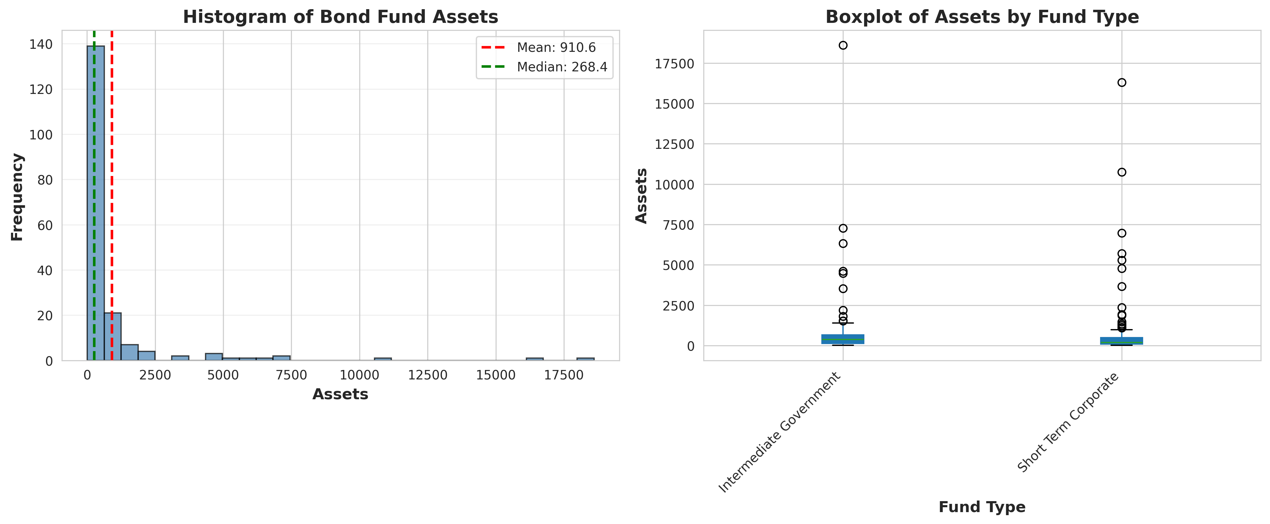
Prompt: Can you provide a histogram of assets and a boxplot of assets by type for the following spreadsheet?

`ChatGPT`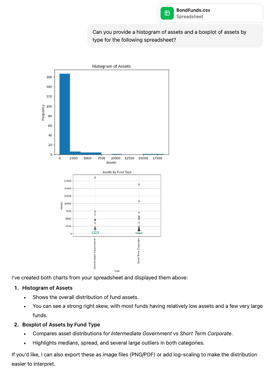

`plotnine`

How’s that done?

import pandas as pd
from plotnine import (
    ggplot, aes, geom_histogram, geom_boxplot,
    labs, theme, element_text, coord_flip
)

df = pd.read_csv('./data/BondFunds.csv')

# Histogram of Assets
hist_plot = (
    ggplot(df, aes(x='Assets'))
    + geom_histogram(bins=30)
    + labs(title='Histogram of Assets', x='Assets', y='Frequency')
)
hist_plot.show()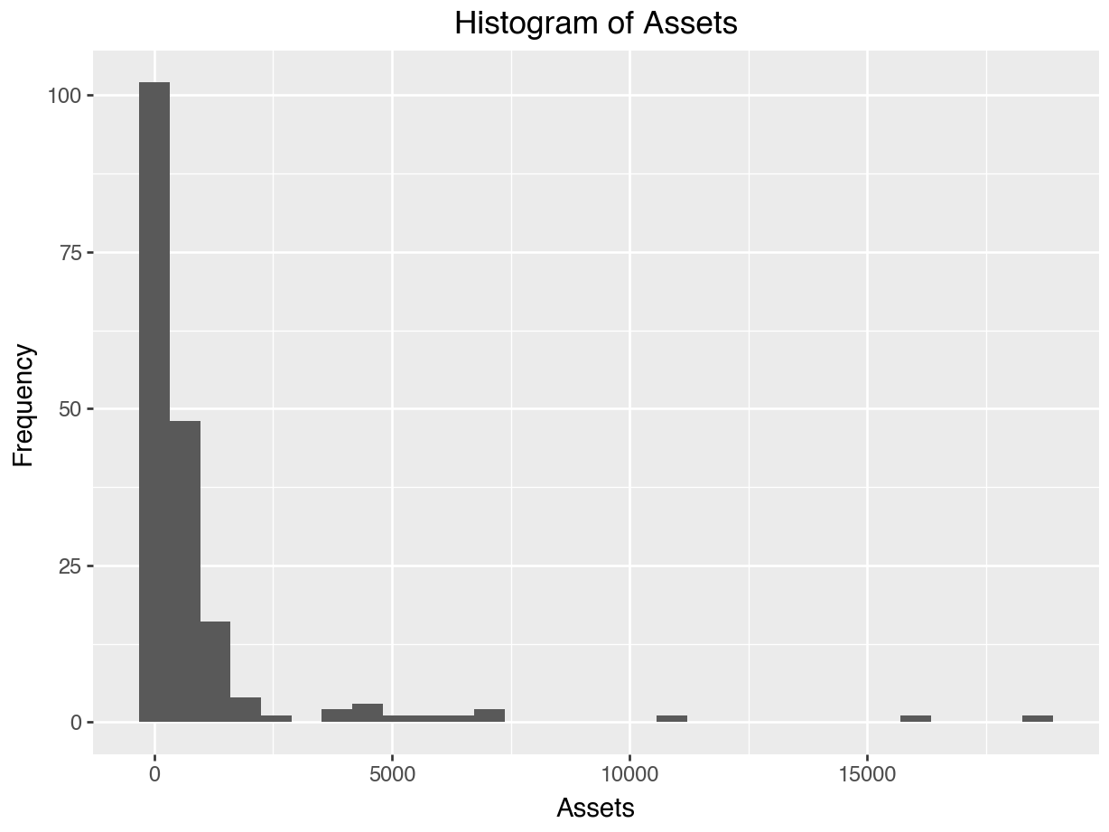

How’s that done?

# Boxplot of Assets by Type
box_plot = (
    ggplot(df, aes(x='Type', y='Assets'))
    + geom_boxplot()
    + labs(title='Assets by Fund Type', x='Type', y='Assets')
    + theme(axis_text_x=element_text(rotation=90, hjust=1)) 
    + coord_flip()
)
box_plot.show()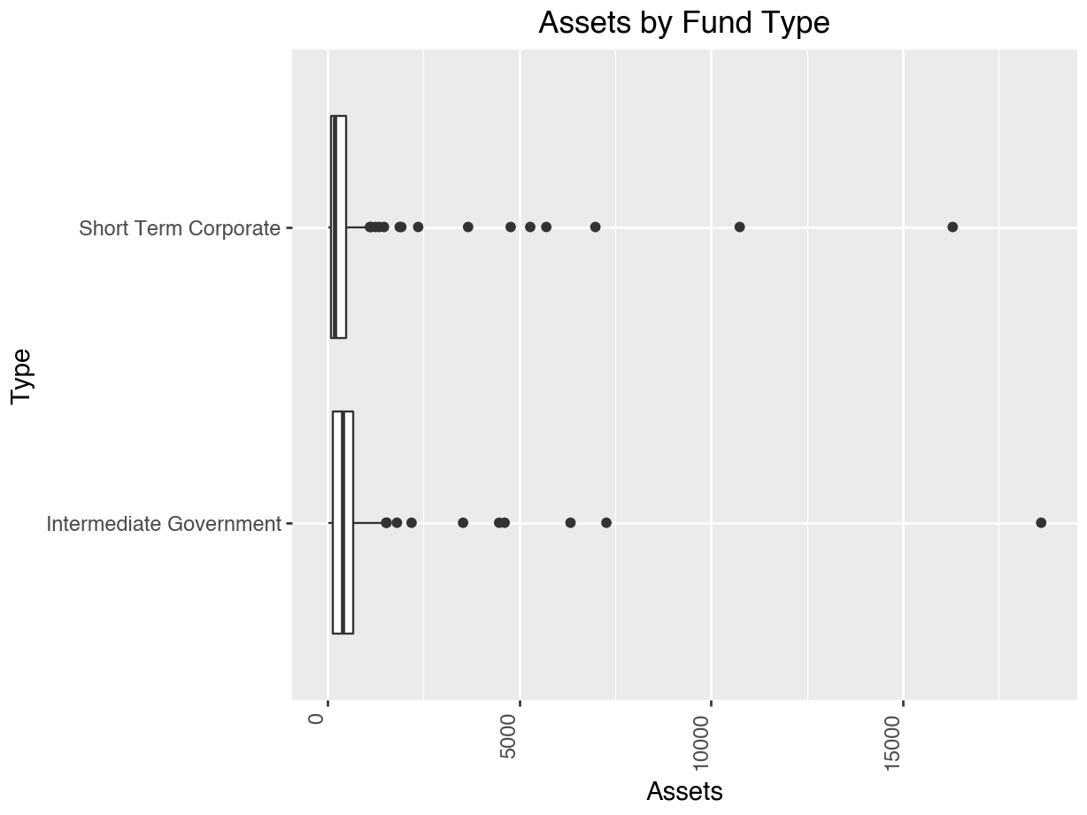

CADDS

The data set presented is designed to represent a sample of 1,000 DDS consumers (which provides a 95% confidence interval with a margin of error of plus-or-minus 3.5% for this 250,000 consumer population). The data set includes six variables (i.e., fields) which are: ID, age cohort/age (binned/unbinned), gender, expenditures, and ethnicity. NB: The data set originated from DDS’s Client Master File. In order to remain in compliance with California State Legislation, the data have been altered to protect the rights and privacy of specific individual consumers. The provided data set is based on actual attributes of consumers.

ID is the unique identification code for each consumer. It is similar to a social security number and used for identification purposes.

Age cohort/age is a key variable in the case exercise. While age is a legal basis for discrimination in many situations, age is not an attribute that would be considered in a discrimination claim for this particular population. The purpose of providing funds to those with developmental disabilities is to help them live like those without disabilities. As consumers get older, their financial needs increase as they move out of their parent’s home, etc. Therefore, it is expected that expenditures for older consumers will be higher than for the younger consumers.

We have included both binned (Age cohort) and unbinned (Age) variables to represent a consumer’s age. The binned age variable is represented in the data set as six age cohorts. Each consumer is assigned to an age cohort based on their years since birth. The six cohorts include: 0-5 years old, 6-12, 13-17, 18-21, 22-50, and 51+. The cohorts are established based on the amount of financial support typically required during a particular life phase.

The 0-5 cohort (preschool age) has the fewest needs and requires the least amount of funding. For the 6-12 cohort (elementary school age) and 13-17 (high school age), a number of needed services are provided by schools. The 18-21 cohort is typically in a transition phase as the consumers begin moving out from their parents’ homes into community centers or living on their own. The majority of those in the 22-50 cohort no longer live with their parents but may still receive some support from their family. Those in the 51+ cohort have the most needs and require the most amount of funding because they are living on their own or in community centers and often have no living parents.

Gender is included in the data set as another variable to consider because it is an attribute on which many discrimination cases are based.

Expenditures variable represents the annual expenditures the State spends on each consumer in supporting these individuals and their families. It is important that students realize this is the amount each consumer receives from the State. Expenditures include services such as: respite for their families, psychological services, medical expenses, transportation, and costs related to housing such as rent (especially for adult consumers living outside their parent’s home).

Ethnicity is the key demographic variable in the data set as it pertains to the case. Eight ethnic groups are represented in the data set. These groups reflect the demographic profile of the State of California. Our key area of interest will become Hispanic and White, non-Hispanic comparisons.

UCB Admissions

Is there evidence of sex bias in admission practices? Data on admissions to the University of California at Berkeley graduate programs in six departments are presented for the population of applicants. Admit measures whether or not the applicant was admitted; M.F measures the [self-reported, two options] gender of the applicant; Dept measures the department in a classification ranging from A to F.

How’s that done?

import pandas as pd

df = pd.read_csv('./data/UCB-Admit.csv')
print(df.head())

    M.F Admit Dept
0  Male   Yes    A
1  Male   Yes    A
2  Male   Yes    A
3  Male   Yes    A
4  Male   Yes    A

How’s that done?

print(df.info())

<class 'pandas.core.frame.DataFrame'>
RangeIndex: 4526 entries, 0 to 4525
Data columns (total 3 columns):
 #   Column  Non-Null Count  Dtype 
---  ------  --------------  ----- 
 0   M.F     4526 non-null   object
 1   Admit   4526 non-null   object
 2   Dept    4526 non-null   object
dtypes: object(3)
memory usage: 106.2+ KB
None

How’s that done?

import matplotlib.pyplot as plt
import seaborn as sns

# Aggregate data
# We want to count occurrences of each (M.F, Admit) pair
counts = df.groupby(['M.F', 'Admit']).size().unstack(fill_value=0)

# Inspect the aggregated data
print(counts)

Admit     No   Yes
M.F               
Female  1278   557
Male    1493  1198

How’s that done?

# Plotting
# X-axis: M.F (Index of counts)
# Stacks: Admit (Columns of counts)
# Using pandas plot kind='bar', stacked=True is easiest

ax = counts.plot(kind='bar', stacked=True, figsize=(10, 6), color=['#d65f5f', '#5fba7d'])
plt.title('Admission Status by Gender')
plt.xlabel('Gender')
plt.ylabel('Count')
plt.xticks(rotation=0)

(array([0, 1]), [Text(0, 0, 'Female'), Text(1, 0, 'Male')])

How’s that done?

plt.legend(title='Admit')
plt.tight_layout()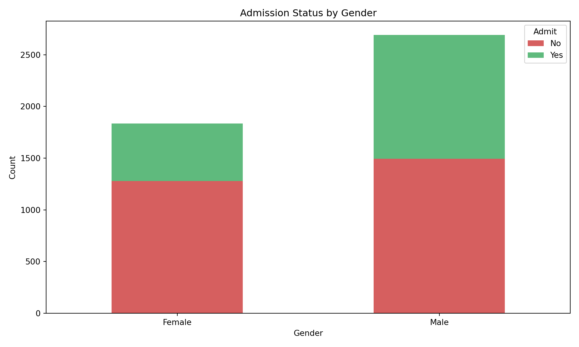

Fast Food

This data has missing values.

How’s that done?

import pandas as pd

# 1. Import the CSV file
url = "./data/FastFood.csv"
df = pd.read_csv(url)

# 2. Count of Missing Values (for all columns)
print("--- Count of Missing Values ---")

--- Count of Missing Values ---

How’s that done?

print(df.isnull().sum())

restaurant       0
item             0
calories         0
cal_fat          0
total_fat        0
sat_fat          0
trans_fat        0
cholesterol      0
sodium           0
total_carb       0
fiber           12
sugar            0
protein          1
vit_a          214
vit_c          210
calcium        210
salad            0
dtype: int64

How’s that done?

print("\n")

How’s that done?

# Filter for numeric columns only for the statistical calculations
numeric_df = df.select_dtypes(include='number')

# 3. Mean
print("--- Mean ---")

--- Mean ---

How’s that done?

print(numeric_df.mean())

calories        530.912621
cal_fat         238.813592
total_fat        26.590291
sat_fat           8.153398
trans_fat         0.465049
cholesterol      72.456311
sodium         1246.737864
total_carb       45.664078
fiber             4.137177
sugar             7.262136
protein          27.891051
vit_a            18.857143
vit_c            20.170492
calcium          24.852459
dtype: float64

How’s that done?

print("\n")

How’s that done?

# 4. Standard Deviation
print("--- Standard Deviation ---")

--- Standard Deviation ---

How’s that done?

print(numeric_df.std())

calories       282.436147
cal_fat        166.407510
total_fat       18.411876
sat_fat          6.418811
trans_fat        0.839644
cholesterol     63.160406
sodium         689.954278
total_carb      24.883342
fiber            3.037460
sugar            6.761301
protein         17.683921
vit_a           31.384330
vit_c           30.592243
calcium         25.522073
dtype: float64

How’s that done?

print("\n")

How’s that done?

# 5. Five Number Summary (Min, Q1, Median, Q3, Max)
# The describe() function includes count, mean, std, and the 5-number summary.
# We will select specific rows to isolate the 5-number summary.
print("--- Five Number Summary ---")

--- Five Number Summary ---

How’s that done?

print(numeric_df.describe().loc[['min', '25%', '50%', '75%', 'max']])

     calories  cal_fat  total_fat  sat_fat  ...  protein  vit_a  vit_c  calcium
min      20.0      0.0        0.0      0.0  ...      1.0    0.0    0.0      0.0
25%     330.0    120.0       14.0      4.0  ...     16.0    4.0    4.0      8.0
50%     490.0    210.0       23.0      7.0  ...     24.5   10.0   10.0     20.0
75%     690.0    310.0       35.0     11.0  ...     36.0   20.0   30.0     30.0
max    2430.0   1270.0      141.0     47.0  ...    186.0  180.0  400.0    290.0

[5 rows x 14 columns]

The class plan:

Pivots and formulae.
Visualizations and types.
Gemini visualizing data. We will use FastFood. Two notes: uploads and missing data

Your assignment for this time:

Do the reading.
From last time. Collect three data visualizations. Think about the approach to visualization presented and how your graphics manifest it. Post them and describe them. What type of data do they represent and how? What is the name of the type of visualization?
For this time, provide three uploaded visualizations. One should use FastFood. The others may use whatever data you wish.

For Next Class:

Reading: Probability
Deliverable: An In-class exercise [Assignment 6] if not completed before departing