How’s that done?
quantile(FastFood$protein, probs = c(0, 0.25, 0.5, 0.75, 1), na.rm = TRUE) 0% 25% 50% 75% 100%
1.0 16.0 24.5 36.0 186.0 Lecture 5: Data Viz I
The arithmetic mean of a variable, call it x, adds up all values of x and divides by the total number:
\[\bar{X}=\frac{1}{n}\sum_{i=1}^nX_i\]
AVERAGE (only count numbers) vs AVERAGEA (count cells).[1] 531[1] 27.9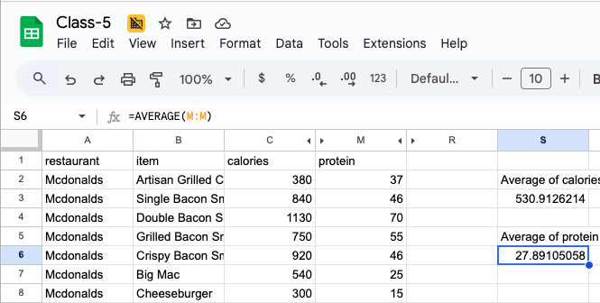
By definition, the sum of the deviations about the average must be zero.
head(FastFood$calories - mean(FastFood$calories))
sum(FastFood$calories - mean(FastFood$calories))[1] -150.91 309.09 599.09 219.09 389.09 9.09[1] 3.41e-12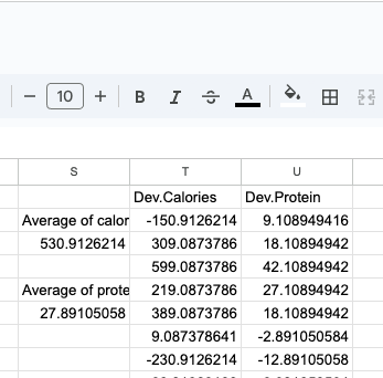
The average is sensitive to outlying values. Think income in Seattle and the samples that include Jeff Bezos, Paul Allen, MacKenzie Scott, and Bill Gates. That is why we examine the median – the value such that half are above and half are below; magnitude doesn’t matter.
The median is a percentile; it is the 50th percentile. We are often also interested in the middle 50 percent: the 25th and 75th percentiles or the first and third quartiles. In R, generically, these are quantiles.
quantile(FastFood$protein, probs = c(0, 0.25, 0.5, 0.75, 1), na.rm = TRUE) 0% 25% 50% 75% 100%
1.0 16.0 24.5 36.0 186.0 As a technical matter, the median is only unique with an odd number of observations; we approximate it with the midpoint of the middle two.
The most frequent or most common value. If it is unique, it is meaningful but it is often not even a small set of values. R doesn’t calculate it. But it is visible in a density or histogram.
With means, we describe the standard deviation. Note, it is singular; it implies the two sides of the center are the same – symmetry. Because the deviations sum to zero, to measure variation, we can’t use untransformed deviation from an average. We work with squares [variance, in the squared metric] or the square root of squares [to maintain the original metric].
\[s=\sqrt{\frac{1}{N-1}\sum_{i=1}^{N}(x_{i}-\overline{x})^2}\]
sd(FastFood$calories)[1] 282We could also work with absolute deviations. The mathematical properties are messier.
We typically measure a range [min to max] or the interquartile range (IQR) – the span of the middle 50%.
quantile(FastFood$calories, probs = c(0, 0.25, 0.5, 0.75, 1)) 0% 25% 50% 75% 100%
20 330 490 690 2430 IQR(FastFood$calories)[1] 360Here it spans 360 calories. The total range is 2410 calories.
transformingIs a key element of radiant used for transforming data. Some of the most common:
It has some nice features.
It fails the simple test of manipulability of the underlying data.
Pre-programmed functions that take input ranges of cells and produce particular outputs.
e.g. set cell J5 to be:
=AVERAGE(C2:C21)This averages the range between C2 and C21 [Assets].

When we copy this left or right, up or down, the numbers and/or letters adjust.
Copy that formula and paste it into K5. Then L5.

Let’s try to make column M into =C2 - J5 , then C3-J5, etc. all the way down to C21.
The 5 won’t stop changing.
We may not want that. Suppose that I want to create a column showing the difference of assets and average assets. In essence, we have rescaled assets such that 0 is the average and we are measuring above or below that average [and by how much]. The $ holds an index constant [F4]. We have two. In our case, we can hold both the rows and the column constant for the average.
Because we are only copying down, the $5 would have sufficed.
=C2 - $J$5
=C2 - J$5
Then copy the formula down to L21. Notice the C changes [no $] but the J doesn’t. The $ enables absolute cell referencing.
As expected. Average assets over the first 20 is 1894.7; the first is 5373.4 above the average for this set.

This can become quite involved; spreadsheets are programming tools. Their underlying problem is that they do not enforce rules or discipline along the way.
The key to our formulae are one or more inputs, a series of transformation and operations, and one or more outputs defined in a precise fashion. Functions link inputs and outputs.
They are models.
Are really cool; they are a very simple and quick way to slice and data and to gain useful comparative and/or summary insight.
They have the added virtue of being drag and drop.

All of the action comes in the calculations shown in the pivot table. Unfortunately, it is extraordinarily limited. Sheets is a bit better.
Excel has probably killed people… recently