The slides are here..

Our ninth class meeting will focus on Chapter 3 and Chapter 4 of Forecasting: Principles and Practice [3rd edition].

All of the data for today, including computations, can be acquired using

load(url("https://github.com/robertwwalker/xaringan/raw/master/CMF-Week-9/data/FullWorkspace.RData"))

Inflation Expectations

```{r}
library(tidyverse)
library(lubridate); library(tsibble)
library(readxl)
url <- "https://www.newyorkfed.org/medialibrary/interactives/sce/sce/downloads/data/frbny-sce-data.xls"
destfile <- "frbny_sce_data.xls"
curl::curl_download(url, destfile)
Inflation.Expectations <- read_excel(destfile, sheet=4, skip=3) %>%
  rename(date = 1) %>% 
  mutate(date = yearmonth(parse_date_time(date, orders = "%Y%m")))
```

```{r}
library(fpp3)
Inflation.Expectations %>% 
  as_tsibble(index=date) %>% 
  autoplot(`Median three-year ahead expected inflation rate`) + 
  geom_line(aes(y=Inflation.Expectations$`Median one-year ahead expected inflation rate`, color="red")) +
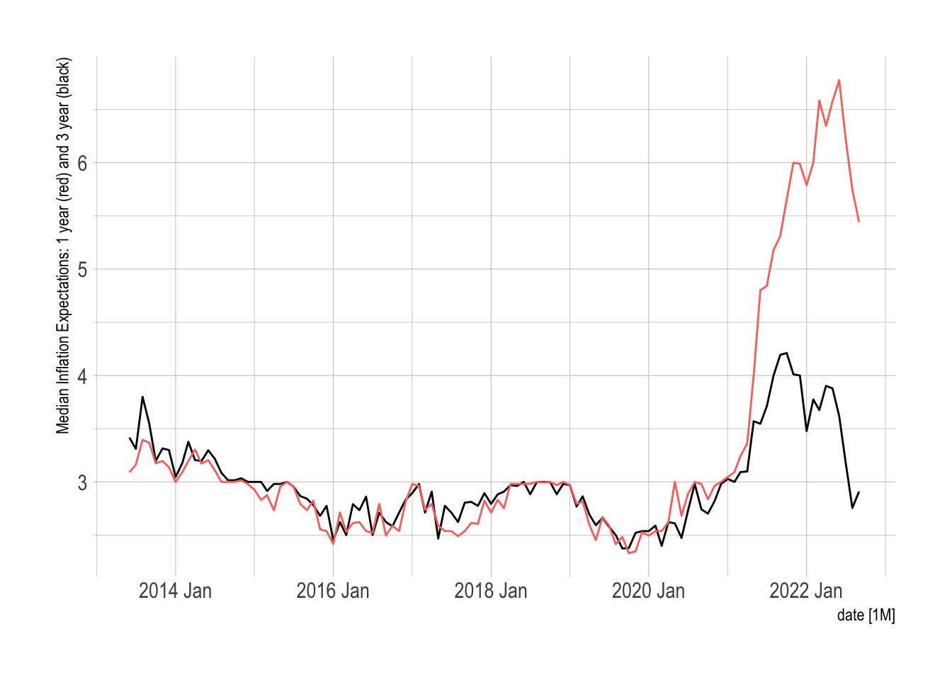
  hrbrthemes::theme_ipsum() + guides(color = "none") + labs(y="Median Inflation Expectations: 1 year (red) and 3 year (black)")
```

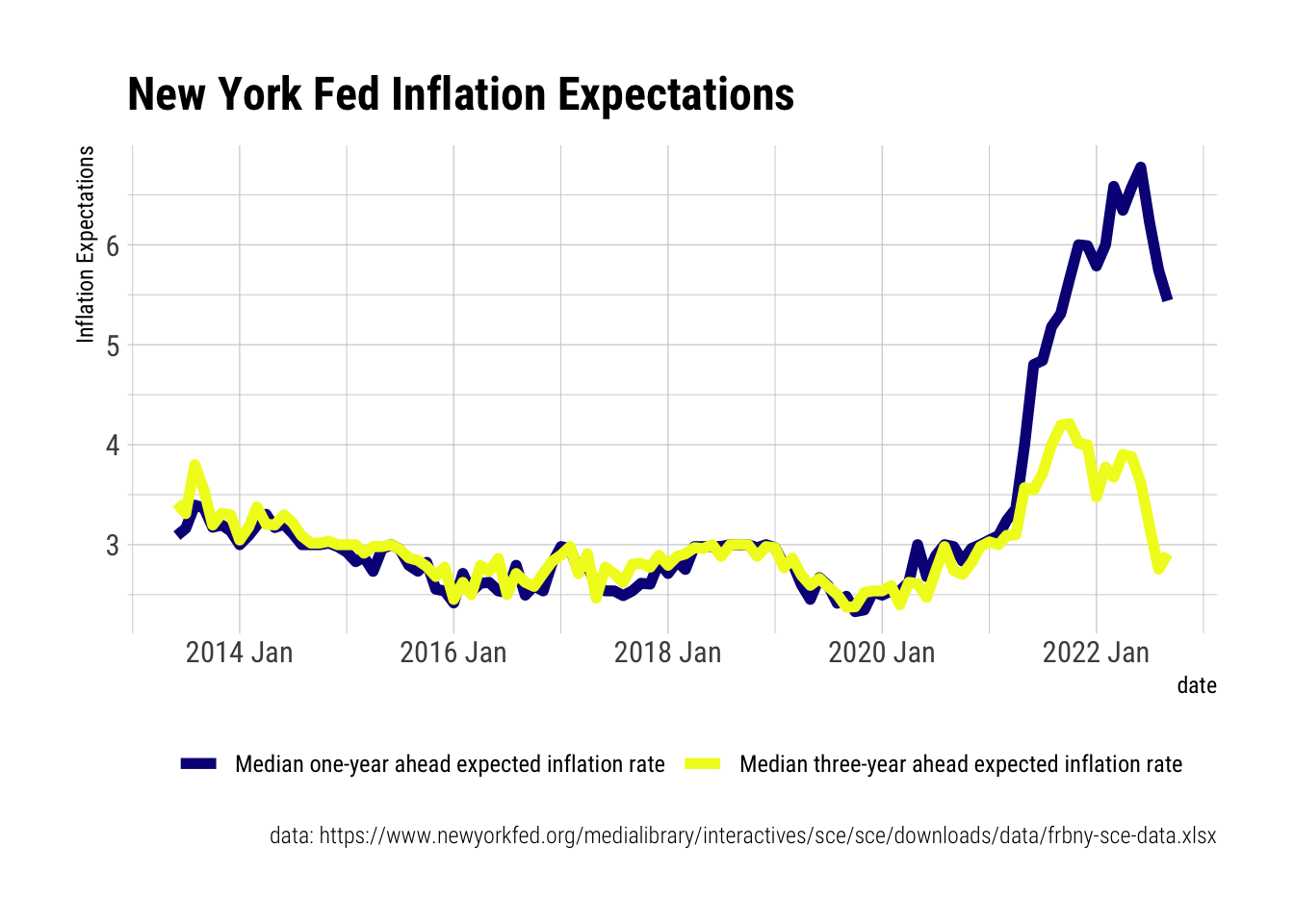
A nicer plot.

```{r}
Inflation.Expectations %>% 
  select(1:3) %>% 
  pivot_longer(c(2:3)) %>%
  mutate(Variable = name) %>%
  ggplot(aes(x=date, y=value, color=Variable)) +
  geom_line(size=2) +
  scale_color_viridis_d(option="C") +
  hrbrthemes::theme_ipsum_rc() +
  theme(legend.position = "bottom") +
  labs(y="Inflation Expectations", 
       color="",
       title="New York Fed Inflation Expectations",
       caption = "data: https://www.newyorkfed.org/medialibrary/interactives/sce/sce/downloads/data/frbny-sce-data.xlsx")
```

Decompositions

Classical Decomposition

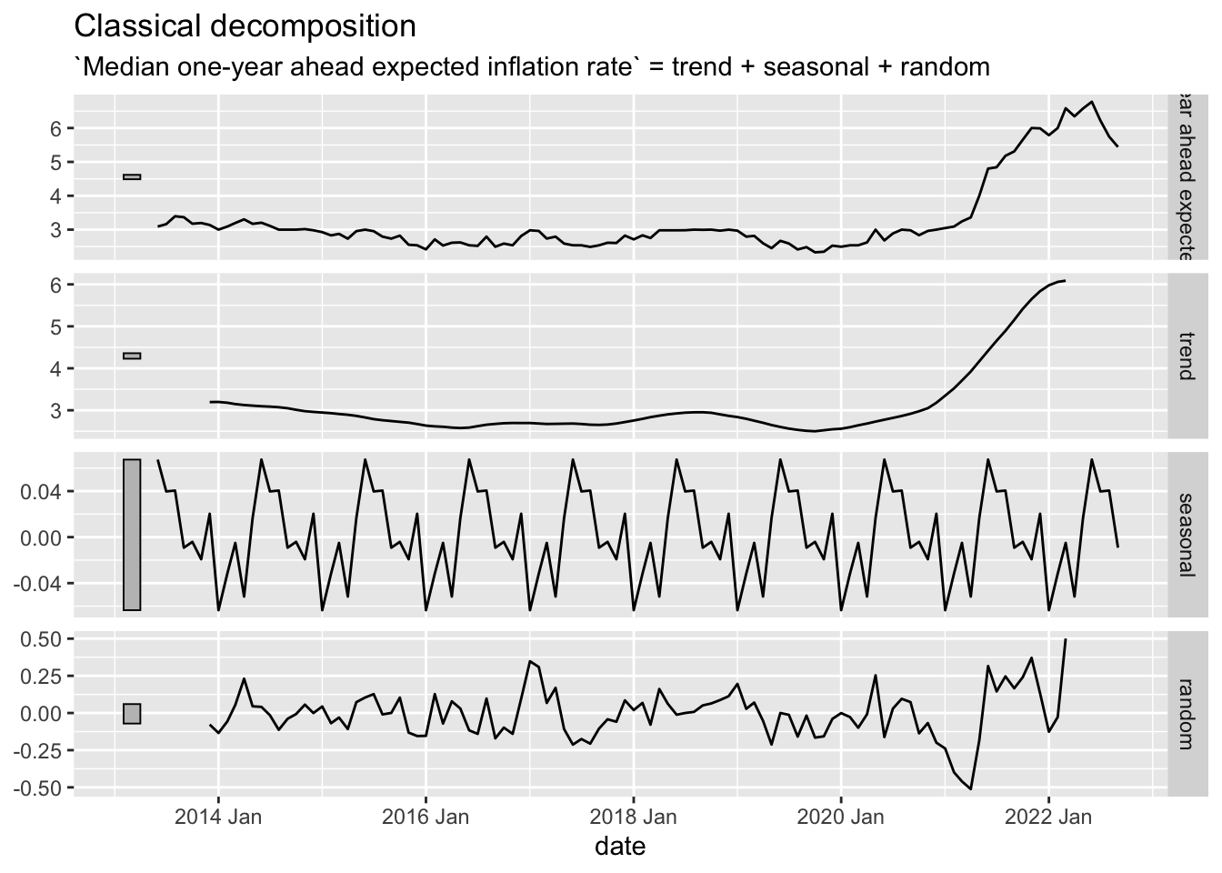
The key difference between the two decompositions, and there are others, is the existence [or lack thereof] of a window. In the classical decomposition, there is almost no flexibility.

```{r}
Inflation.Expectations %>% 
  as_tsibble(index=date) %>% 
  model(stl = classical_decomposition(`Median one-year ahead expected inflation rate` ~ season(12))) %>%
  components() %>% 
  autoplot()
```

STL Decomposition

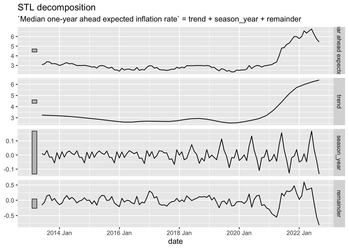
The key new element to the STL decomposition is the window argument. Over how many time periods should the trend/season be calculated. If one wishes to average over all periods, window="periodic" is the necessary syntax.

```{r}
Inflation.Expectations %>% 
  as_tsibble(index=date) %>% 
  model(STL(`Median one-year ahead expected inflation rate`)) %>%
  components() %>% 
  autoplot()
```