Code
library(flextable); library(tidyverse); library(webshot2)
Model.Cars <- lm(dist ~ speed, data=cars)
as_flextable(Model.Cars) %>% theme_vanilla() %>% save_as_image("img/RegTable.png", webshot = "webshot2")Robert W. Walker
February 6, 2023
Meeting Date: February 6, 2023.
Last updated: 2023-04-10 13:52:56
Timezone: America/Los_Angeles
gtflextableThe fourth assignment consists of adding at two production quality tables to your portfolio. One in the gt or flextable style. One using DT::datatable

Deliverables: an email containing the URLs for the table posts.
I made a comment in the syllabus that is not quite right. stargazer is indeed nice for producing publication quality tables. But flextable can do this too.
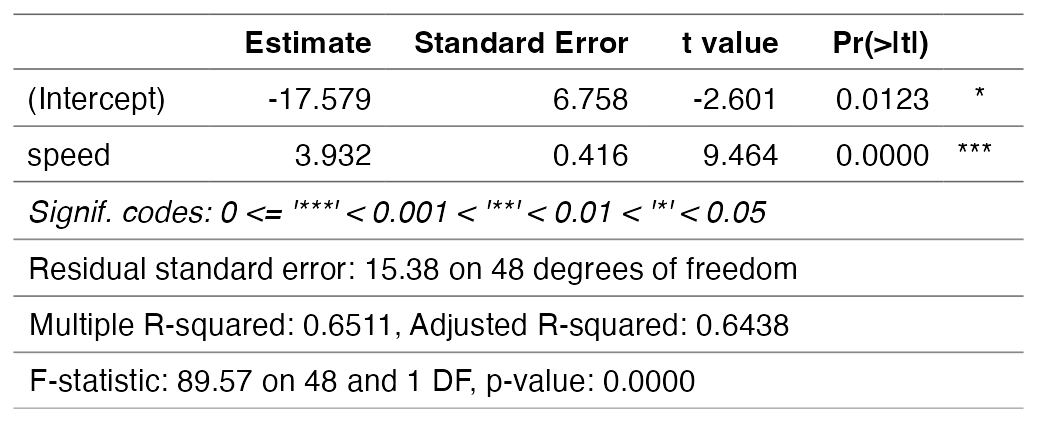
The base render doesn’t work with the dark theme.
Estimate | Standard Error | t value | Pr(>|t|) | ||
|---|---|---|---|---|---|
(Intercept) | -17.579 | 6.758 | -2.601 | 0.0123 | * |
speed | 3.932 | 0.416 | 9.464 | 0.0000 | *** |
Signif. codes: 0 <= '***' < 0.001 < '**' < 0.01 < '*' < 0.05 | |||||
Residual standard error: 15.38 on 48 degrees of freedom | |||||
Multiple R-squared: 0.6511, Adjusted R-squared: 0.6438 | |||||
F-statistic: 89.57 on 48 and 1 DF, p-value: 0.0000 | |||||
use_df_printer()
Bonds <- read.csv(url("https://raw.githubusercontent.com/robertwwalker/DADMStuff/master/BondFunds.csv"), row.names = 1)
obj <- summarizor(Bonds, by = "Risk", overall_label = "Overall")
obj
Above average | Average | Below average | Overall | ||||||
|---|---|---|---|---|---|---|---|---|---|
Type | Intermediate Government | 29 (49.15%) | 32 (46.38%) | 26 (46.43%) | 87 (47.28%) | ||||
Short Term Corporate | 30 (50.85%) | 37 (53.62%) | 30 (53.57%) | 97 (52.72%) | |||||
Missing | 0 (0.00%) | 0 (0.00%) | 0 (0.00%) | 0 (0.00%) | |||||
Assets | Mean (SD) | 969.4 (2558.1) | 965.8 (2432.8) | 780.8 (1628.0) | 910.6 (2253.3) | ||||
Median (IQR) | 278.4 (537.8) | 298.1 (557.2) | 232.4 (440.0) | 268.4 (508.2) | |||||
Range | 12.4 - 16297.1 | 17.3 - 18603.5 | 17.4 - 7268.1 | 12.4 - 18603.5 | |||||
Missing | 0 (0.00%) | 0 (0.00%) | 0 (0.00%) | 0 (0.00%) | |||||
Fees | No | 37 (62.71%) | 49 (71.01%) | 44 (78.57%) | 130 (70.65%) | ||||
Yes | 22 (37.29%) | 20 (28.99%) | 12 (21.43%) | 54 (29.35%) | |||||
Missing | 0 (0.00%) | 0 (0.00%) | 0 (0.00%) | 0 (0.00%) | |||||
Expense.Ratio | Mean (SD) | 0.7 (0.3) | 0.7 (0.2) | 0.7 (0.2) | 0.7 (0.3) | ||||
Median (IQR) | 0.7 (0.4) | 0.7 (0.4) | 0.7 (0.3) | 0.7 (0.4) | |||||
Range | 0.1 - 1.9 | 0.1 - 1.6 | 0.3 - 1.1 | 0.1 - 1.9 | |||||
Missing | 0 (0.00%) | 0 (0.00%) | 0 (0.00%) | 0 (0.00%) | |||||
Return.2009 | Mean (SD) | 8.3 (9.2) | 6.9 (4.4) | 6.3 (2.7) | 7.2 (6.1) | ||||
Median (IQR) | 7.9 (13.0) | 6.0 (7.3) | 6.1 (3.2) | 6.4 (7.2) | |||||
Range | -8.8 - 32.0 | -1.1 - 16.4 | 0.2 - 13.0 | -8.8 - 32.0 | |||||
Missing | 0 (0.00%) | 0 (0.00%) | 0 (0.00%) | 0 (0.00%) | |||||
X3.Year.Return | Mean (SD) | 4.2 (3.8) | 5.0 (1.5) | 4.8 (1.6) | 4.7 (2.5) | ||||
Median (IQR) | 5.5 (3.5) | 5.4 (1.5) | 5.0 (2.2) | 5.1 (2.0) | |||||
Range | -13.8 - 9.4 | 0.4 - 7.3 | -0.2 - 7.5 | -13.8 - 9.4 | |||||
Missing | 0 (0.00%) | 0 (0.00%) | 0 (0.00%) | 0 (0.00%) | |||||
X5.Year.Return | Mean (SD) | 3.6 (2.2) | 4.2 (1.0) | 4.1 (0.9) | 4.0 (1.5) | ||||
Median (IQR) | 4.3 (2.0) | 4.4 (1.2) | 4.1 (1.3) | 4.3 (1.3) | |||||
Range | -7.3 - 6.8 | 1.5 - 6.2 | 1.8 - 6.1 | -7.3 - 6.8 | |||||
Missing | 0 (0.00%) | 0 (0.00%) | 0 (0.00%) | 0 (0.00%) |
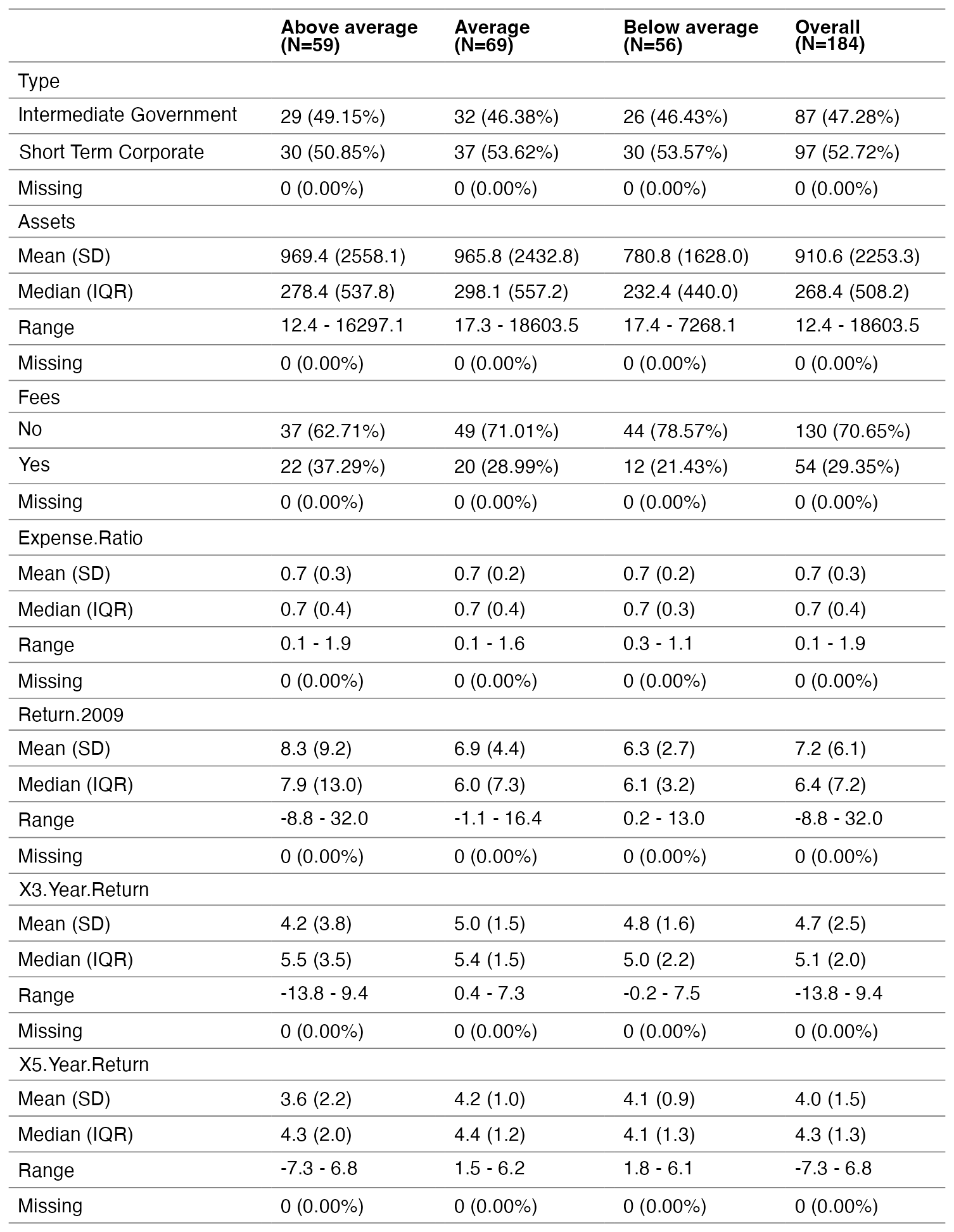
Above average | Average | Below average | Overall | |||||
|---|---|---|---|---|---|---|---|---|
Type | ||||||||
Intermediate Government | 29 (49.15%) | 32 (46.38%) | 26 (46.43%) | 87 (47.28%) | ||||
Short Term Corporate | 30 (50.85%) | 37 (53.62%) | 30 (53.57%) | 97 (52.72%) | ||||
Missing | 0 (0.00%) | 0 (0.00%) | 0 (0.00%) | 0 (0.00%) | ||||
Assets | ||||||||
Mean (SD) | 969.4 (2558.1) | 965.8 (2432.8) | 780.8 (1628.0) | 910.6 (2253.3) | ||||
Median (IQR) | 278.4 (537.8) | 298.1 (557.2) | 232.4 (440.0) | 268.4 (508.2) | ||||
Range | 12.4 - 16297.1 | 17.3 - 18603.5 | 17.4 - 7268.1 | 12.4 - 18603.5 | ||||
Missing | 0 (0.00%) | 0 (0.00%) | 0 (0.00%) | 0 (0.00%) | ||||
Fees | ||||||||
No | 37 (62.71%) | 49 (71.01%) | 44 (78.57%) | 130 (70.65%) | ||||
Yes | 22 (37.29%) | 20 (28.99%) | 12 (21.43%) | 54 (29.35%) | ||||
Missing | 0 (0.00%) | 0 (0.00%) | 0 (0.00%) | 0 (0.00%) | ||||
Expense.Ratio | ||||||||
Mean (SD) | 0.7 (0.3) | 0.7 (0.2) | 0.7 (0.2) | 0.7 (0.3) | ||||
Median (IQR) | 0.7 (0.4) | 0.7 (0.4) | 0.7 (0.3) | 0.7 (0.4) | ||||
Range | 0.1 - 1.9 | 0.1 - 1.6 | 0.3 - 1.1 | 0.1 - 1.9 | ||||
Missing | 0 (0.00%) | 0 (0.00%) | 0 (0.00%) | 0 (0.00%) | ||||
Return.2009 | ||||||||
Mean (SD) | 8.3 (9.2) | 6.9 (4.4) | 6.3 (2.7) | 7.2 (6.1) | ||||
Median (IQR) | 7.9 (13.0) | 6.0 (7.3) | 6.1 (3.2) | 6.4 (7.2) | ||||
Range | -8.8 - 32.0 | -1.1 - 16.4 | 0.2 - 13.0 | -8.8 - 32.0 | ||||
Missing | 0 (0.00%) | 0 (0.00%) | 0 (0.00%) | 0 (0.00%) | ||||
X3.Year.Return | ||||||||
Mean (SD) | 4.2 (3.8) | 5.0 (1.5) | 4.8 (1.6) | 4.7 (2.5) | ||||
Median (IQR) | 5.5 (3.5) | 5.4 (1.5) | 5.0 (2.2) | 5.1 (2.0) | ||||
Range | -13.8 - 9.4 | 0.4 - 7.3 | -0.2 - 7.5 | -13.8 - 9.4 | ||||
Missing | 0 (0.00%) | 0 (0.00%) | 0 (0.00%) | 0 (0.00%) | ||||
X5.Year.Return | ||||||||
Mean (SD) | 3.6 (2.2) | 4.2 (1.0) | 4.1 (0.9) | 4.0 (1.5) | ||||
Median (IQR) | 4.3 (2.0) | 4.4 (1.2) | 4.1 (1.3) | 4.3 (1.3) | ||||
Range | -7.3 - 6.8 | 1.5 - 6.2 | 1.8 - 6.1 | -7.3 - 6.8 | ||||
Missing | 0 (0.00%) | 0 (0.00%) | 0 (0.00%) | 0 (0.00%) | ||||
Borrowed from Ted Laderas.
Ted Laderas [@laderast on Twitter] wrote a function to present the ten most expensive items in a category for the items dataset. You can find his repo for this here.. I will change rows 3 and 9. Line 3 adds the new argument to the function and line 9 carries the variable defined in the argument into top_n.
library(ggimage); library(gt)
library(tidyverse)
most_expensive <- function(category_name=NULL, price_category=buy_value){
  if(!is.null(category_name)){
    items <- items %>%
      filter(category == category_name)
  }
items %>%
  top_n(10, {{price_category}}) %>%
  arrange(desc({{price_category}})) %>%
  select(name, sell_value, buy_value, category, image=image_url) %>%
  gt() %>%
   text_transform(
    locations = cells_body(vars(image)),
    fn = function(x) {
      web_image(
        url = x,
        height = 50
      )
    }
  )
}library(ggimage); library(gt)
library(tidyverse)
most_expensive <- function(category_name=NULL, price_category=buy_value, n=10){
if(!is.null(category_name)){
items <- items %>%
filter(category == category_name)
}
items %>%
top_n(n, {{price_category}}) %>%
arrange(desc({{price_category}})) %>%
select(name, image=image_url, sell_value, buy_value, category) %>%
gt() %>%
text_transform(
locations = cells_body(vars(image)),
fn = function(x) {
web_image(
url = x,
height = 50
)
}
)
}most_expensive() %>%
tab_header(title = "Most Expensive Items in Animal Crossing By Buy Price") %>%
cols_label(
name = "Item",
sell_value = "Sale Price",
buy_value = "Buy Price",
category = "Item Type",
image = "Picture"
) %>% tab_spanner(
label = "Prices",
columns = c(buy_value, sell_value)
)| Most Expensive Items in Animal Crossing By Buy Price | ||||
| Item | Picture | Prices | Item Type | |
|---|---|---|---|---|
| Buy Price | Sale Price | |||
| Royal Crown |  |
1200000 | 300000 | Hats |
| Crown |  |
1000000 | 250000 | Hats |
| Gold Armor |  |
320000 | 80000 | Dresses |
| Golden Casket |  |
320000 | 80000 | Furniture |
| Grand Piano |  |
260000 | 65000 | Furniture |
| Golden Toilet |  |
240000 | 60000 | Furniture |
| Blue Steel Staircase |  |
228000 | NA | Furniture |
| Iron Bridge |  |
228000 | NA | Furniture |
| Red Steel Staircase |  |
228000 | NA | Furniture |
| Red Zen Bridge |  |
228000 | NA | Furniture |
| Zen Bridge |  |
228000 | NA | Furniture |
most_expensive("Hats") %>%  tab_header(title = "Most Expensive Items in Animal Crossing By Buy Price") %>%  cols_label(
    name = "Item",
    sell_value = "Sale Price",
    buy_value = "Buy Price",
    category = "Item Type",
    image = "Picture"
) %>%   tab_spanner(
    label = "Prices",
    columns = c(buy_value, sell_value)
)| Most Expensive Items in Animal Crossing By Buy Price | ||||
| Item | Picture | Prices | Item Type | |
|---|---|---|---|---|
| Buy Price | Sale Price | |||
| Royal Crown |  |
1200000 | 300000 | Hats |
| Crown |  |
1000000 | 250000 | Hats |
| Gold Helmet |  |
200000 | 50000 | Hats |
| Blue Rose Crown |  |
48000 | 12000 | Hats |
| Gold Rose Crown |  |
48000 | 12000 | Hats |
| Snowperson Head |  |
28000 | 7000 | Hats |
| Knight's Helmet |  |
15000 | 3750 | Hats |
| Dark Cosmos Crown |  |
13440 | 3360 | Hats |
| Chic Rose Crown |  |
11520 | 2880 | Hats |
| Purple Hyacinth Crown | 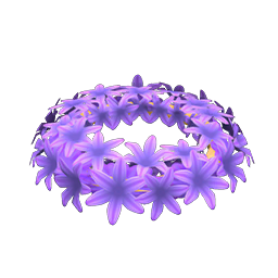 |
11520 | 2880 | Hats |
| Purple Pansy Crown |  |
11520 | 2880 | Hats |
| Purple Windflower Crown |  |
11520 | 2880 | Hats |
| Simple Mum Crown |  |
11520 | 2880 | Hats |
most_expensive("Fossils", price_category = sell_value, n=65) %>%  tab_header(title = "Most Expensive Items in Animal Crossing By Buy Price") %>%  cols_label(
    name = "Item",
    sell_value = "Sale Price",
    buy_value = "Buy Price",
    category = "Item Type",
    image = "Picture"
) %>%   tab_spanner(
    label = "Prices",
    columns = c(buy_value, sell_value)
)| Most Expensive Items in Animal Crossing By Buy Price | ||||
| Item | Picture | Prices | Item Type | |
|---|---|---|---|---|
| Buy Price | Sale Price | |||
| Brachio Skull |  |
NA | 6000 | Fossils |
| T. Rex Skull |  |
NA | 6000 | Fossils |
| Brachio Chest |  |
NA | 5500 | Fossils |
| Brachio Tail | 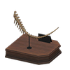 |
NA | 5500 | Fossils |
| Dimetrodon Skull | 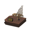 |
NA | 5500 | Fossils |
| Right Megalo Side | 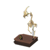 |
NA | 5500 | Fossils |
| T. Rex Torso | 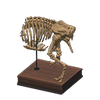 |
NA | 5500 | Fossils |
| Tricera Skull | 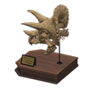 |
NA | 5500 | Fossils |
| Brachio Pelvis | 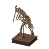 |
NA | 5000 | Fossils |
| Dimetrodon Torso | 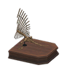 |
NA | 5000 | Fossils |
| Diplo Skull | 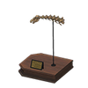 |
NA | 5000 | Fossils |
| Diplo Tail | 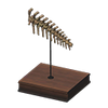 |
NA | 5000 | Fossils |
| Left Quetzal Wing | 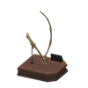 |
NA | 5000 | Fossils |
| Right Quetzal Wing |  |
NA | 5000 | Fossils |
| Stego Skull | 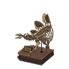 |
NA | 5000 | Fossils |
| T. Rex Tail | 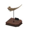 |
NA | 5000 | Fossils |
| Tricera Torso | 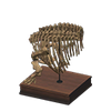 |
NA | 5000 | Fossils |
| Diplo Neck | 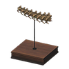 |
NA | 4500 | Fossils |
| Diplo Pelvis | 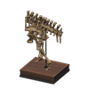 |
NA | 4500 | Fossils |
| Left Ptera Wing | 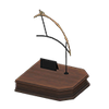 |
NA | 4500 | Fossils |
| Megacero Skull | 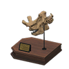 |
NA | 4500 | Fossils |
| Plesio Body | 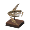 |
NA | 4500 | Fossils |
| Plesio Tail |  |
NA | 4500 | Fossils |
| Quetzal Torso |  |
NA | 4500 | Fossils |
| Right Ptera Wing | 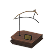 |
NA | 4500 | Fossils |
| Stego Torso |  |
NA | 4500 | Fossils |
| Tricera Tail | 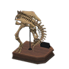 |
NA | 4500 | Fossils |
| Archelon Skull |  |
NA | 4000 | Fossils |
| Diplo Chest | 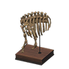 |
NA | 4000 | Fossils |
| Diplo Tail Tip |  |
NA | 4000 | Fossils |
| Iguanodon Skull |  |
NA | 4000 | Fossils |
| Left Megalo Side | 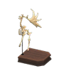 |
NA | 4000 | Fossils |
| Pachy Skull | 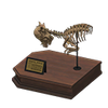 |
NA | 4000 | Fossils |
| Plesio Skull | 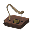 |
NA | 4000 | Fossils |
| Ptera Body | 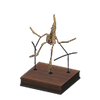 |
NA | 4000 | Fossils |
| Spino Skull | 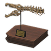 |
NA | 4000 | Fossils |
| Stego Tail |  |
NA | 4000 | Fossils |
| Ankylo Skull |  |
NA | 3500 | Fossils |
| Archelon Tail |  |
NA | 3500 | Fossils |
| Dunkleosteus |  |
NA | 3500 | Fossils |
| Iguanodon Torso | 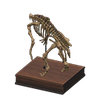 |
NA | 3500 | Fossils |
| Megacero Torso | 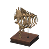 |
NA | 3500 | Fossils |
| Pachy Tail |  |
NA | 3500 | Fossils |
| Parasaur Skull |  |
NA | 3500 | Fossils |
| Ankylo Torso | 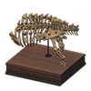 |
NA | 3000 | Fossils |
| Deinony Torso |  |
NA | 3000 | Fossils |
| Iguanodon Tail | 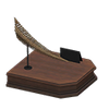 |
NA | 3000 | Fossils |
| Mammoth Skull |  |
NA | 3000 | Fossils |
| Megacero Tail | 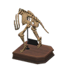 |
NA | 3000 | Fossils |
| Parasaur Torso | 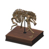 |
NA | 3000 | Fossils |
| Spino Torso | 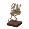 |
NA | 3000 | Fossils |
| Ankylo Tail | 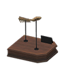 |
NA | 2500 | Fossils |
| Deinony Tail |  |
NA | 2500 | Fossils |
| Mammoth Torso |  |
NA | 2500 | Fossils |
| Ophthalmo Skull |  |
NA | 2500 | Fossils |
| Opthalmo Skull |  |
NA | 2500 | Fossils |
| Opthalmo Torso |  |
NA | 2500 | Fossils |
| Parasaur Tail |  |
NA | 2500 | Fossils |
| Sabertooth Skull |  |
NA | 2500 | Fossils |
| Spino Tail | 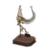 |
NA | 2500 | Fossils |
| Acanthostega | 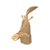 |
NA | 2000 | Fossils |
| Anomalocaris | 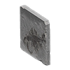 |
NA | 2000 | Fossils |
| Eusthenopteron |  |
NA | 2000 | Fossils |
| Ophthalmo Torso | 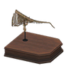 |
NA | 2000 | Fossils |
| Sabertooth Tail |  |
NA | 2000 | Fossils |