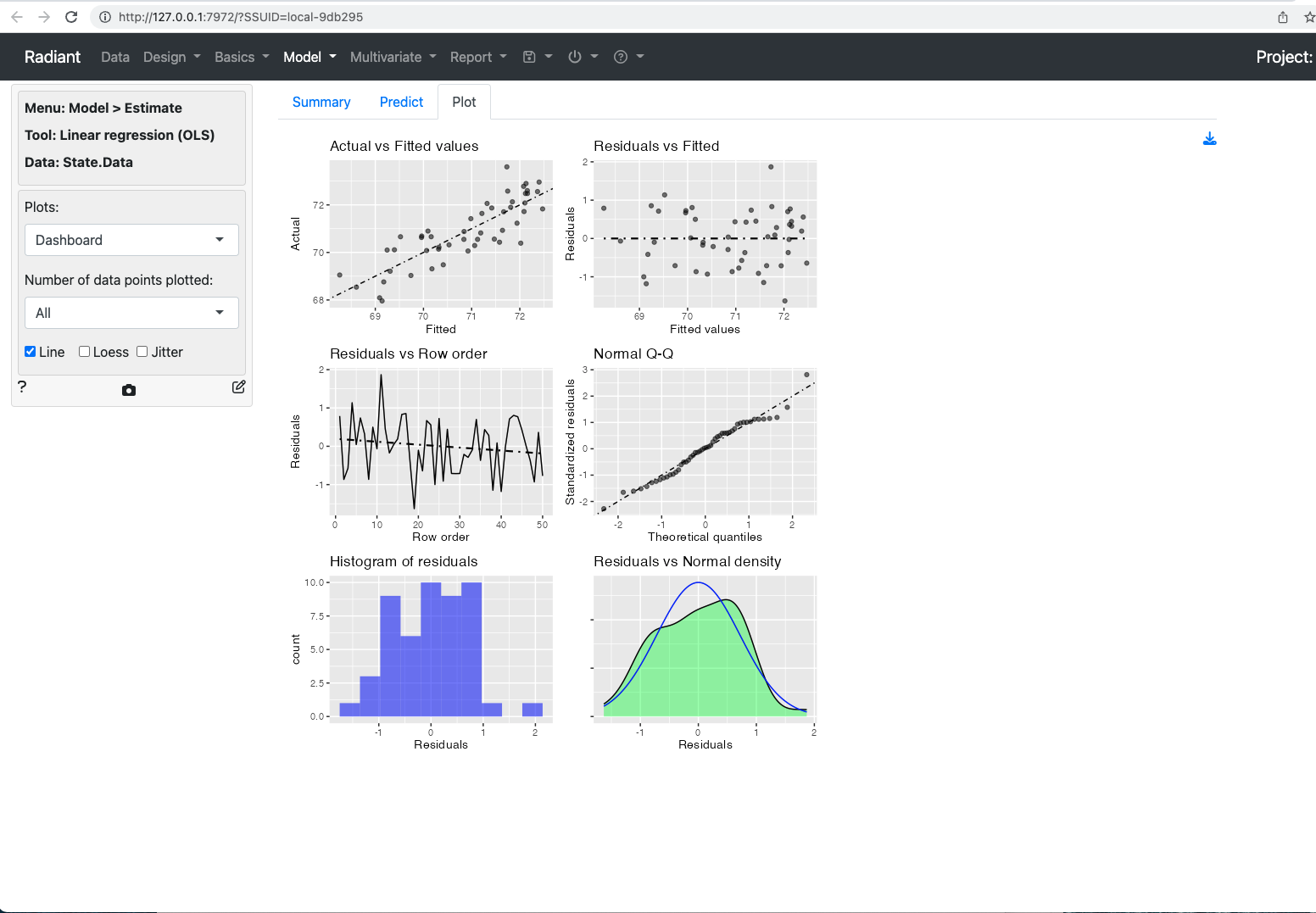
Data Analysis, Modelling, and Decision-Making

radiant is a very convenient graphical interface for a curated subset of R’s capabilities. In this example, I show how to incorporate additional code into radiant to examine residual normality as a component of validating regression inference.

Let us first begin with some example data. We can read the data off of the github host location for this website.

library(tidyverse)
State.Data <- read_csv(url("https://raw.githubusercontent.com/robertwwalker/DADM-FAQ/main/posts/normal-residuals-in-radiant/data/state77.csv"))
State.Data

# A tibble: 50 × 9
   state       population income illiteracy life_exp murder hs_grad frost   area
   <chr>            <dbl>  <dbl>      <dbl>    <dbl>  <dbl>   <dbl> <dbl>  <dbl>
 1 Alabama           3615   3624        2.1     69.0   15.1    41.3    20  50708
 2 Alaska             365   6315        1.5     69.3   11.3    66.7   152 566432
 3 Arizona           2212   4530        1.8     70.6    7.8    58.1    15 113417
 4 Arkansas          2110   3378        1.9     70.7   10.1    39.9    65  51945
 5 California       21198   5114        1.1     71.7   10.3    62.6    20 156361
 6 Colorado          2541   4884        0.7     72.1    6.8    63.9   166 103766
 7 Connecticut       3100   5348        1.1     72.5    3.1    56     139   4862
 8 Delaware           579   4809        0.9     70.1    6.2    54.6   103   1982
 9 Florida           8277   4815        1.3     70.7   10.7    52.6    11  54090
10 Georgia           4931   4091        2       68.5   13.9    40.6    60  58073
# … with 40 more rows

You can access the radiant state file here.

Regression Dialog

I want a regression to illustrate, let me try to explain life_exp or life expectancy.

We need to make sure we write the code to the report by using the scribe button just below and to the right of +Store.

Press the button and the resulting code will appear in the Report tab in radiant under Rmd.

library(radiant)
result <- regress(
  State.Data, 
  rvar = "life_exp", 
  evar = c("population", "income", "illiteracy", "murder", "hs_grad")
)
summary(result)

Knit the report to see the following output.

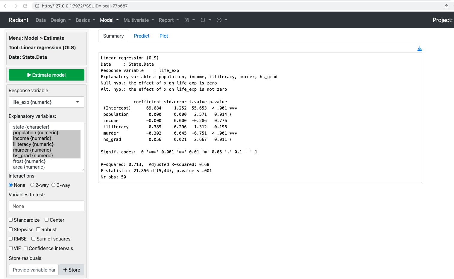
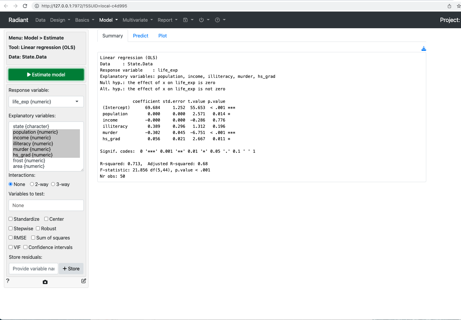
Linear regression (OLS)
Data     : State.Data 
Response variable    : life_exp 
Explanatory variables: population, income, illiteracy, murder, hs_grad 
Null hyp.: the effect of x on life_exp is zero
Alt. hyp.: the effect of x on life_exp is not zero

             coefficient std.error t.value p.value    
 (Intercept)      69.684     1.252  55.653  < .001 ***
 population        0.000     0.000   2.571   0.014 *  
 income           -0.000     0.000  -0.286   0.776    
 illiteracy        0.389     0.296   1.312   0.196    
 murder           -0.302     0.045  -6.751  < .001 ***
 hs_grad           0.056     0.021   2.667   0.011 *  

Signif. codes:  0 '***' 0.001 '**' 0.01 '*' 0.05 '.' 0.1 ' ' 1

R-squared: 0.713,  Adjusted R-squared: 0.68 
F-statistic: 21.856 df(5,44), p.value < .001
Nr obs: 50

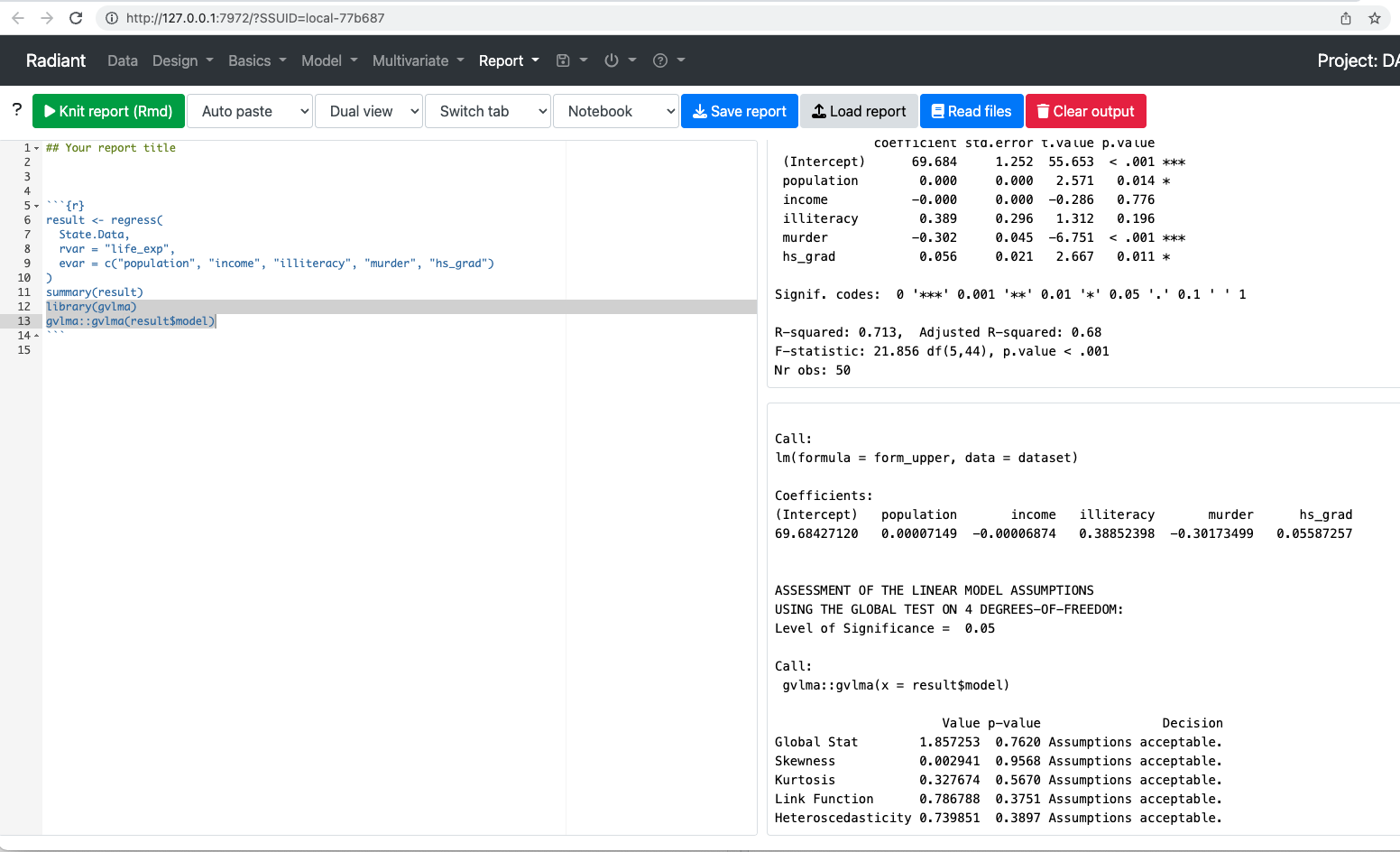
gvlma

To investigate residuals using radiant, we need to first call a library. The library is gvlma or general validation of linear model assumptions. The necessary command is library(gvlma). Then we want to call gvlma on the model. In this case, that is gvlma(result$model).

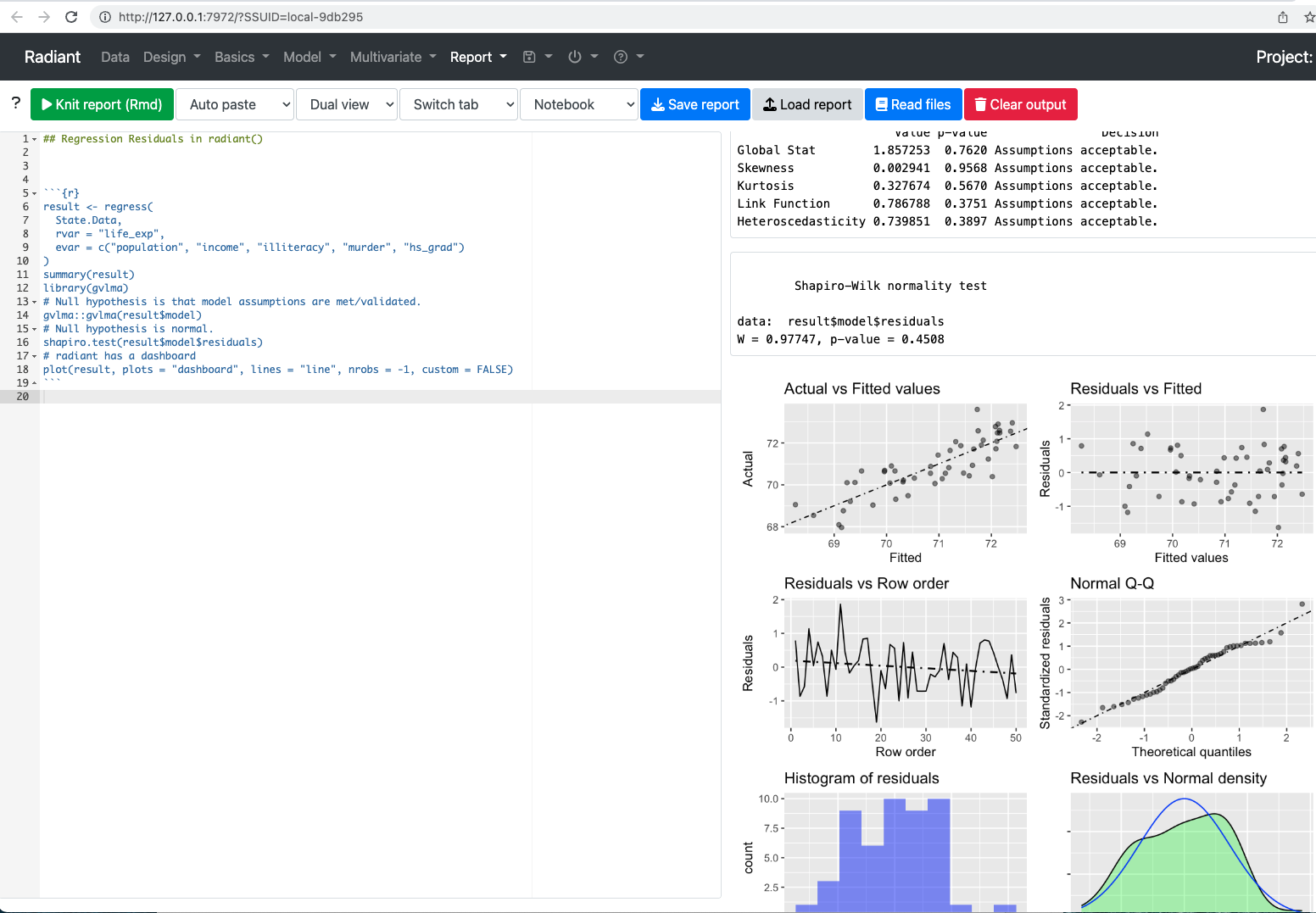
Once we have added the code, click knit report and the following output should result.

library(gvlma)
gvlma::gvlma(result$model)


Call:
lm(formula = form_upper, data = dataset)

Coefficients:
(Intercept)   population       income   illiteracy       murder      hs_grad  
  6.968e+01    7.149e-05   -6.874e-05    3.885e-01   -3.017e-01    5.587e-02  


ASSESSMENT OF THE LINEAR MODEL ASSUMPTIONS
USING THE GLOBAL TEST ON 4 DEGREES-OF-FREEDOM:
Level of Significance =  0.05 

Call:
 gvlma::gvlma(x = result$model) 

                      Value p-value                Decision
Global Stat        1.857253  0.7620 Assumptions acceptable.
Skewness           0.002941  0.9568 Assumptions acceptable.
Kurtosis           0.327674  0.5670 Assumptions acceptable.
Link Function      0.786788  0.3751 Assumptions acceptable.
Heteroscedasticity 0.739851  0.3897 Assumptions acceptable.

There are reasons to prefer gvlma but we could also use a few other tools. We could deploy a command that requires no additional libraries. With a null hypothesis that residuals are normal and recognizing this is probably best in cases like this with only fifty observations.

shapiro.test(result$model$residuals)


    Shapiro-Wilk normality test

data:  result$model$residuals
W = 0.97747, p-value = 0.4508

We could also use plotlyreg with the requisite packages installed. I don’t currently like this because it fails to pass the axis names.

source(url("https://github.com/robertwwalker/DADMStuff/raw/master/PlotlyReg.R"))
RegressionPlots(result$model)

radiant() also has a nice internal dashboard for assessing this.

That can be added to the report by clicking on the pencil/tablet.