Pivoting Data: Long and Wide

R
Author

Robert W. Walker

Published

September 12, 2020

Pivoting Data

The ability to pivot data from long to wide format or from wide to long format is one of the greatest time saving devices that I know of. Let’s first look at the data types: wide and long.

Wide Data

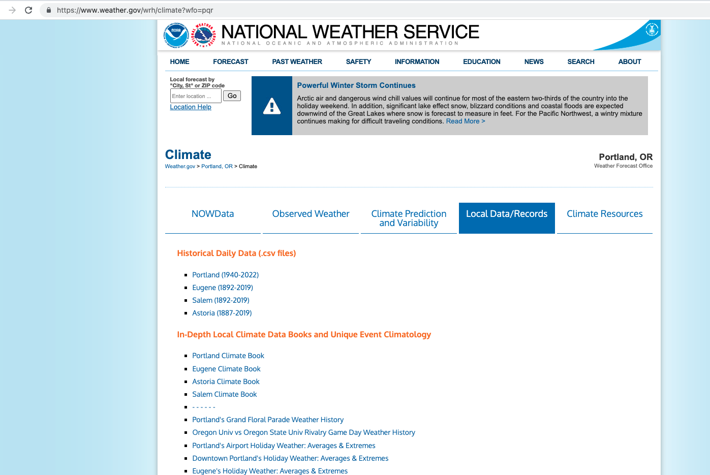
I will use climate data covering the city of Portland from the National Weather Service. [The data were obtained from:] (https://w2.weather.gov/climate/local_data.php?wfo=pqr) and you will notice that there are data for Astoria, Salem and Eugene, also. Notice this is the Local Data and Records tab.

ScreenShot

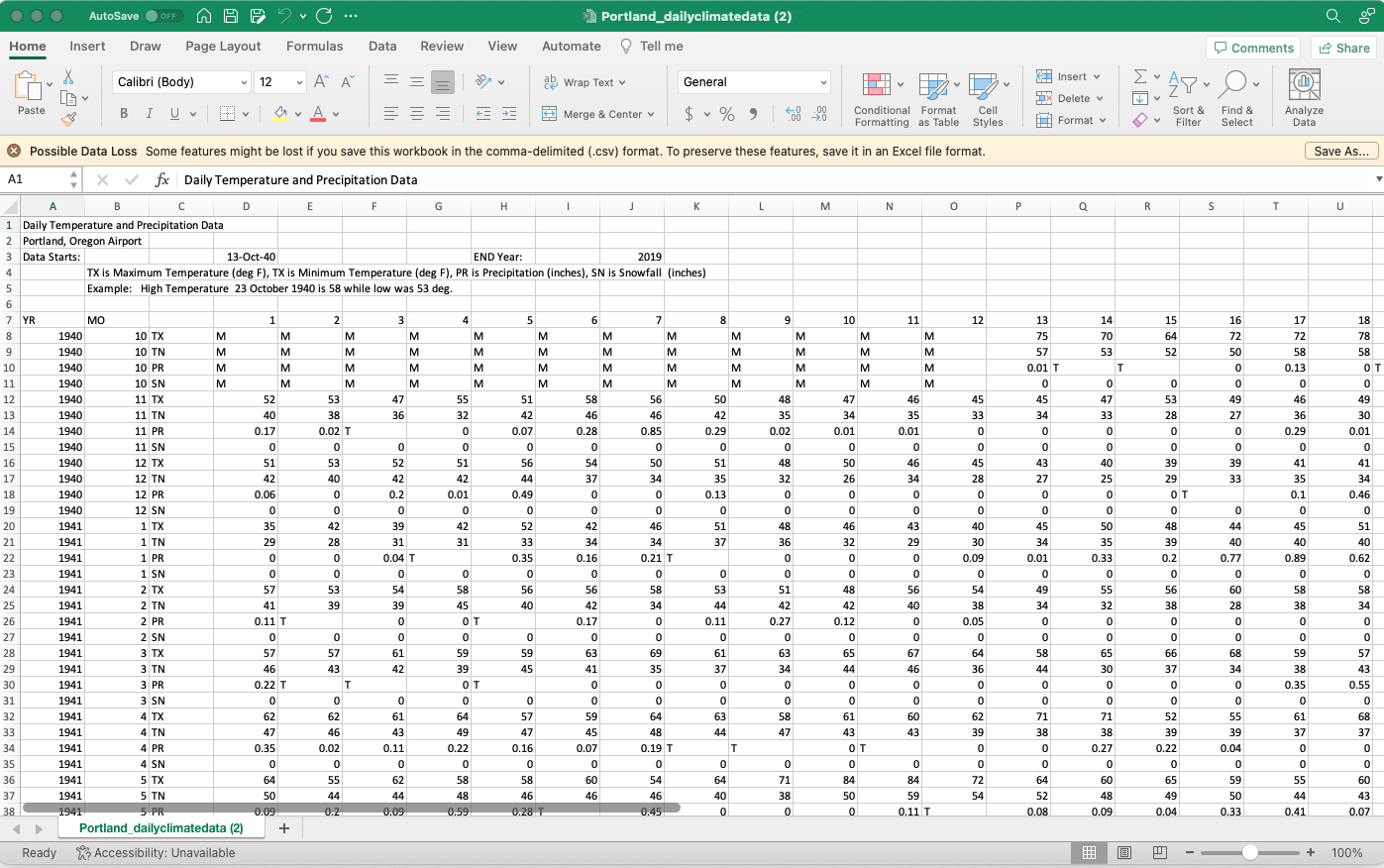
I downloaded the Portland data and examined the spreadsheet. It has a rather straightforward wide structure – it has data in the column names. Other common examples are accounting data with the variables listed as rows and the time periods as the columns.

NWS Spreadsheet

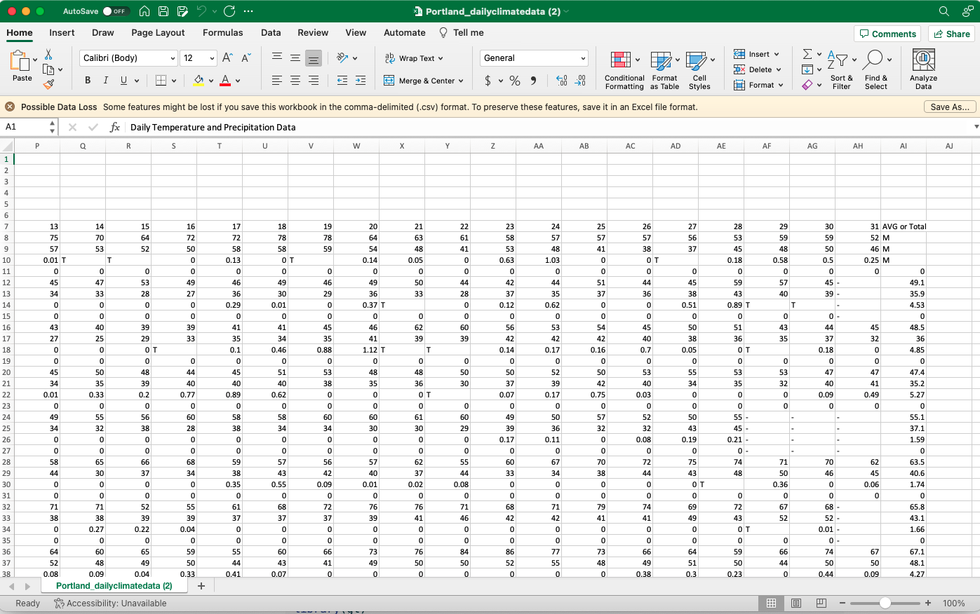
There are a few rows describing the data that will have to be eliminated to import the data; that’s the skip flag so I will use skip=6. If we examine row 7, we will see what will become the variable names. YR and MO are year and month, respectively, there is then a blank and the remaining names are the day; it extends to 31. For each month, there are four rows representing the high TX, the low TN, precipitation PR, and snow SN. Scrolling rightward, we see the remainder of the spreadsheet from the image above; there is also an AVG or Total column.

NWS Spreadsheet

Were I to import them as is, let’s see what happens just skipping the first six rows. I will use the gt package to show what I have.

library(tidyverse)
library(gt)
NWS <- read.csv(url("https://www.weather.gov/source/pqr/climate/webdata/Portland_dailyclimatedata.csv"), skip=6)
head(NWS, 10) %>% gt()
YR MO X X1 X2 X3 X4 X5 X6 X7 X8 X9 X10 X11 X12 X13 X14 X15 X16 X17 X18 X19 X20 X21 X22 X23 X24 X25 X26 X27 X28 X29 X30 X31 AVG.or.Total
1940 10 TX M M M M M M M M M M M M 75 70 64 72 72 78 78 64 63 61 58 57 57 57 56 53 59 59 52 M
1940 10 TN M M M M M M M M M M M M 57 53 52 50 58 58 59 54 48 41 53 48 41 38 37 45 48 50 46 M
1940 10 PR M M M M M M M M M M M M 0.01 T T 0 0.13 0 T 0.14 0.05 0 0.63 1.03 0 0 T 0.18 0.58 0.5 0.25 M
1940 10 SN M M M M M M M M M M M M 0 0 0 0 0 0 0 0 0 0 0 0 0 0 0 0 0 0 0 0
1940 11 TX 52 53 47 55 51 58 56 50 48 47 46 45 45 47 53 49 46 49 46 49 50 44 42 44 51 44 45 59 57 45 - 49.1
1940 11 TN 40 38 36 32 42 46 46 42 35 34 35 33 34 33 28 27 36 30 29 36 33 28 37 35 37 36 38 43 40 39 - 35.9
1940 11 PR 0.17 0.02 T 0 0.07 0.28 0.85 0.29 0.02 0.01 0.01 0 0 0 0 0 0.29 0.01 0 0.37 T 0 0.12 0.62 0 0 0.51 0.89 T T - 4.53
1940 11 SN 0 0 0 0 0 0 0 0 0 0 0 0 0 0 0 0 0 0 0 0 0 0 0 0 0 0 0 0 0 0 - 0
1940 12 TX 51 53 52 51 56 54 50 51 48 50 46 45 43 40 39 39 41 41 45 46 62 60 56 53 54 45 50 51 43 44 45 48.5
1940 12 TN 42 40 42 42 44 37 34 35 32 26 34 28 27 25 29 33 35 34 35 41 39 39 42 42 42 40 38 36 35 37 32 36

That is a pretty good start. There are a few types of missing data (the M values) and some conversions to consider before I can start. There are some - for days that do not exist. T stands for Trace amount, the lowest recorded numeric values are 0.01 inches. There are also values labelled as T/A which I assume to be Trace/Accumulation because there is no obvious dictionary describing their exact meanings.

Let’s start by reflecting a skip of the first six rows and two sets of missing values, M and -. I also want to rename the column that has no name in the original spreadsheet to be Variable because this is that column reflecting which of the four actual variables that we have for the month-year combination.

NWS <- read.csv(url("https://www.weather.gov/source/pqr/climate/webdata/Portland_dailyclimatedata.csv"), 
                skip=6, 
                na.strings = c("M","-", "")) %>% 
  rename(Variable = X)
head(NWS, 10) %>% gt()
YR MO Variable X1 X2 X3 X4 X5 X6 X7 X8 X9 X10 X11 X12 X13 X14 X15 X16 X17 X18 X19 X20 X21 X22 X23 X24 X25 X26 X27 X28 X29 X30 X31 AVG.or.Total
1940 10 TX NA NA NA NA NA NA NA NA NA NA NA NA 75 70 64 72 72 78 78 64 63 61 58 57 57 57 56 53 59 59 52 NA
1940 10 TN NA NA NA NA NA NA NA NA NA NA NA NA 57 53 52 50 58 58 59 54 48 41 53 48 41 38 37 45 48 50 46 NA
1940 10 PR NA NA NA NA NA NA NA NA NA NA NA NA 0.01 T T 0 0.13 0 T 0.14 0.05 0 0.63 1.03 0 0 T 0.18 0.58 0.5 0.25 NA
1940 10 SN NA NA NA NA NA NA NA NA NA NA NA NA 0 0 0 0 0 0 0 0 0 0 0 0 0 0 0 0 0 0 0 0
1940 11 TX 52 53 47 55 51 58 56 50 48 47 46 45 45 47 53 49 46 49 46 49 50 44 42 44 51 44 45 59 57 45 NA 49.1
1940 11 TN 40 38 36 32 42 46 46 42 35 34 35 33 34 33 28 27 36 30 29 36 33 28 37 35 37 36 38 43 40 39 NA 35.9
1940 11 PR 0.17 0.02 T 0 0.07 0.28 0.85 0.29 0.02 0.01 0.01 0 0 0 0 0 0.29 0.01 0 0.37 T 0 0.12 0.62 0 0 0.51 0.89 T T NA 4.53
1940 11 SN 0 0 0 0 0 0 0 0 0 0 0 0 0 0 0 0 0 0 0 0 0 0 0 0 0 0 0 0 0 0 NA 0
1940 12 TX 51 53 52 51 56 54 50 51 48 50 46 45 43 40 39 39 41 41 45 46 62 60 56 53 54 45 50 51 43 44 45 48.5
1940 12 TN 42 40 42 42 44 37 34 35 32 26 34 28 27 25 29 33 35 34 35 41 39 39 42 42 42 40 38 36 35 37 32 36

I can handle the T/A values by just removing the /A that appears in a few places.

NWS <- NWS %>% 
  mutate(across(where(is.character), 
                ~str_remove(.x, "/A")))

The T values still exist and but this will be enough to avail us of easy access to some monthly data for a first pivot example after eliminating one additional problem. The data end in December 2019.

NWS %>% tail(n = 10) %>% gt()
YR MO Variable X1 X2 X3 X4 X5 X6 X7 X8 X9 X10 X11 X12 X13 X14 X15 X16 X17 X18 X19 X20 X21 X22 X23 X24 X25 X26 X27 X28 X29 X30 X31 AVG.or.Total
2019 11 PR 0 0 0 0 T 0 0 0 0.19 0.05 0 0.17 0 0 0.13 T 0.08 0.11 0.49 0 0 0 0 0.16 0.05 0.09 0 0 0 T NA 1.52
2019 11 SN 0 0 0 0 0 0 0 0 0 0 0 0 0 0 0 0 0 0 0 0 0 0 0 0 0 0 0 0 0 T NA T
2019 12 TX 43 47 49 50 53 50 46 53 49 45 47 54 49 47 44 48 42 43 57 59 51 46 48 40 44 46 45 48 48 48 51 48.1
2019 12 TN 35 30 32 38 39 38 43 45 38 38 42 45 40 40 37 36 35 32 38 50 43 42 35 32 31 27 37 40 40 40 40 38
2019 12 PR 0.12 0 0 T 0 0.25 0.46 T 0 0.32 0.29 0.31 0 0.03 0 T 0 0.18 0.64 0.4 0.88 0.17 0.09 T 0.02 T 0.01 0 T 0 0.22 4.39
2019 12 SN 0 0 0 0 0 0 0 0 0 0 0 0 0 0 0 0 0 0 0 0 0 0 0 0 0 0 0 0 0 0 0 0
2020 1 TX NA NA NA NA NA NA NA NA NA NA NA NA NA NA NA NA NA NA NA NA NA NA NA NA NA NA NA NA NA NA NA NA
2020 1 TN NA NA NA NA NA NA NA NA NA NA NA NA NA NA NA NA NA NA NA NA NA NA NA NA NA NA NA NA NA NA NA NA
2020 1 PR NA NA NA NA NA NA NA NA NA NA NA NA NA NA NA NA NA NA NA NA NA NA NA NA NA NA NA NA NA NA NA NA
2020 1 SN NA NA NA NA NA NA NA NA NA NA NA NA NA NA NA NA NA NA NA NA NA NA NA NA NA NA NA NA NA NA NA NA

I want to filter those rows out.

NWS <- NWS %>% filter(!(MO==1 & YR==2020)) 
NWS %>% tail(n=10) %>% gt()
YR MO Variable X1 X2 X3 X4 X5 X6 X7 X8 X9 X10 X11 X12 X13 X14 X15 X16 X17 X18 X19 X20 X21 X22 X23 X24 X25 X26 X27 X28 X29 X30 X31 AVG.or.Total
2019 10 PR 0 T 0.02 0.06 0 0 0.08 0.02 0 0 T 0 0 0 T 0.37 0.28 0.02 0.43 0.03 0.01 0.15 0 0 0.04 T 0 0 T 0 0 1.51
2019 10 SN 0 0 0 0 0 0 0 0 0 0 0 0 0 0 0 0 0 0 0 0 0 0 0 0 0 0 0 0 0 0 0 0
2019 11 TX 62 63 59 54 49 66 62 62 51 55 62 52 53 57 58 56 56 58 55 58 57 50 50 51 51 44 47 44 45 45 NA 54.4
2019 11 TN 31 33 37 37 35 43 37 37 40 48 44 45 44 43 44 46 49 52 47 40 34 32 31 40 41 41 37 37 26 26 NA 39.2
2019 11 PR 0 0 0 0 T 0 0 0 0.19 0.05 0 0.17 0 0 0.13 T 0.08 0.11 0.49 0 0 0 0 0.16 0.05 0.09 0 0 0 T NA 1.52
2019 11 SN 0 0 0 0 0 0 0 0 0 0 0 0 0 0 0 0 0 0 0 0 0 0 0 0 0 0 0 0 0 T NA T
2019 12 TX 43 47 49 50 53 50 46 53 49 45 47 54 49 47 44 48 42 43 57 59 51 46 48 40 44 46 45 48 48 48 51 48.1
2019 12 TN 35 30 32 38 39 38 43 45 38 38 42 45 40 40 37 36 35 32 38 50 43 42 35 32 31 27 37 40 40 40 40 38
2019 12 PR 0.12 0 0 T 0 0.25 0.46 T 0 0.32 0.29 0.31 0 0.03 0 T 0 0.18 0.64 0.4 0.88 0.17 0.09 T 0.02 T 0.01 0 T 0 0.22 4.39
2019 12 SN 0 0 0 0 0 0 0 0 0 0 0 0 0 0 0 0 0 0 0 0 0 0 0 0 0 0 0 0 0 0 0 0

From here I should be able to build some monthly data.

Monthly Data.

I want to pick out four columns from which to build dates for the data; let’s work on a monthly time series. Because the sum or average is already a column, I do not need to create it. I only need select it.

# Now to create a Monthly time series.
NWS.Monthly.Base <- NWS %>% 
  select(YR, MO, Variable, AVG.or.Total)

I will use a pipe from the magrittr package to reduce typing. %<>% substitutes for a combination of <- and %>% to update the object that I am operating on. I have some character values in that column and the original picture of the wide end of the data shows a missing average/total for October 1940; the T values are replaced by 0.005.

library(magrittr)
NWS.Monthly.Base %<>% filter(!(MO==10 & YR==1940)) %>%
  mutate(AVG.or.Total = recode(AVG.or.Total, T = "0.005"))

From there, I will use pivot_wider to move Variable to columns and their names and taking the values of each from the average/total column. How does it look?

NWS.Monthly.Tidy <- NWS.Monthly.Base %>%  
  pivot_wider(names_from = "Variable", 
              values_from = "AVG.or.Total")
NWS.Monthly.Tidy %>% head() %>% gt()
YR MO TX TN PR SN
1940 11 49.1 35.9 4.53 0
1940 12 48.5 36 4.85 0
1941 1 47.4 35.2 5.27 0
1941 2 55.1 37.1 1.59 0
1941 3 63.5 40.6 1.74 0
1941 4 65.8 43.1 1.66 0

Let me put together a date using paste and lubridate’s year-month format.

library(lubridate)
NWS.Monthly.Tidy %<>%  mutate(Month.Yr =
                                ym(paste(YR,MO, sep="-")))

What about turning them numeric?

NWS.Monthly.Tidy %<>%  mutate(High = as.numeric(TX), 
         Low = as.numeric(TN), 
         Precipitation = as.numeric(PR), 
         Snow = as.numeric(SN)
         ) %>%
  select(Month.Yr, High, Low, Precipitation, Snow)
NWS.Monthly.Tidy %>% head(n=10) %>% gt()
Month.Yr High Low Precipitation Snow
1940-11-01 49.1 35.9 4.53 0
1940-12-01 48.5 36.0 4.85 0
1941-01-01 47.4 35.2 5.27 0
1941-02-01 55.1 37.1 1.59 0
1941-03-01 63.5 40.6 1.74 0
1941-04-01 65.8 43.1 1.66 0
1941-05-01 67.1 48.1 4.27 0
1941-06-01 71.6 52.6 0.81 0
1941-07-01 84.5 58.3 0.03 0
1941-08-01 77.6 58.0 1.45 0

That’s exactly what I need. To treat it as a functional time series, let me deploy the fpp3 package, tsibble requires the specification of a time index and these are monthly data but they are tidy, rows represent the units [periods of time] and the columns are variables. This is a time series because one of them is time.

library(fpp3)
NWS.Monthly.TS <- NWS.Monthly.Tidy %>% 
  mutate(YM = yearmonth(Month.Yr)) %>%
  as_tsibble(index=YM)

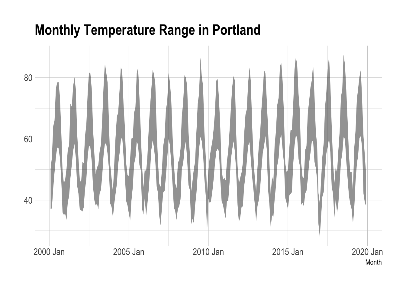
To see the fluctuation in high and low temperatures from 2000 to 2019, we can show it.

library(hrbrthemes)
NWS.Monthly.TS %>% 
  filter(Month.Yr > as.Date("2000-01-01")) %>% 
  ggplot() + 
  aes(x=YM) + 
  geom_ribbon(aes(ymin=Low, ymax=High), alpha=0.5) + 
  theme_ipsum() +
  labs(title="Monthly Temperature Range in Portland",
       x="Month")

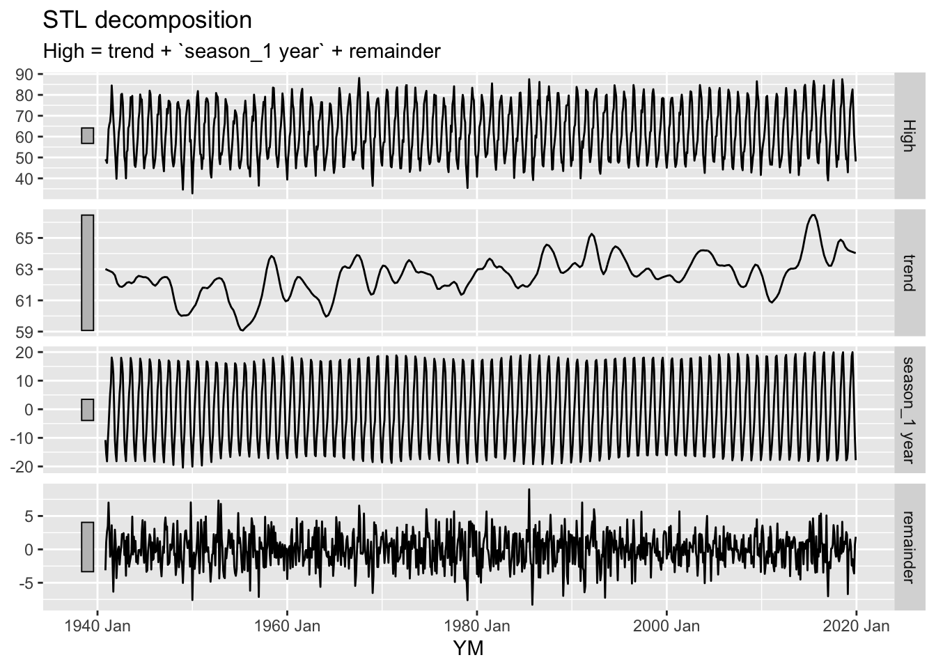
Because it is enabled, what does the STL decomposition suggest for temperature change; let’s look at the high temperatures.

NWS.Monthly.TS %>% 
  model(STL(High ~ season(period="1 year") + trend(window=30, degree=0))) %>% 
  components() %>% 
  autoplot()

A Summary of the Monthly Data

The key feature is spreading out the row for each initial variable in the pivot command and then clearing out the messy values. To turn it into a monthly time series, fpp3 has the yearmonth data structure.

Daily Data

Let me start with the original data and a single column omission, I want to get rid of the monthly total/average column and start some daily data.

NWS.Daily <- NWS %>% select(-AVG.or.Total)
names(NWS.Daily) <- c("YR","MO","Variable",paste0("Day.",1:31))
head(NWS.Daily)
    YR MO Variable Day.1 Day.2 Day.3 Day.4 Day.5 Day.6 Day.7 Day.8 Day.9 Day.10
1 1940 10       TX  <NA>  <NA>  <NA>  <NA>  <NA>  <NA>  <NA>  <NA>  <NA>   <NA>
2 1940 10       TN  <NA>  <NA>  <NA>  <NA>  <NA>  <NA>  <NA>  <NA>  <NA>   <NA>
3 1940 10       PR  <NA>  <NA>  <NA>  <NA>  <NA>  <NA>  <NA>  <NA>  <NA>   <NA>
4 1940 10       SN  <NA>  <NA>  <NA>  <NA>  <NA>  <NA>  <NA>  <NA>  <NA>   <NA>
5 1940 11       TX    52    53    47    55    51    58    56    50    48     47
6 1940 11       TN    40    38    36    32    42    46    46    42    35     34
  Day.11 Day.12 Day.13 Day.14 Day.15 Day.16 Day.17 Day.18 Day.19 Day.20 Day.21
1   <NA>   <NA>     75     70     64     72     72     78     78     64     63
2   <NA>   <NA>     57     53     52     50     58     58     59     54     48
3   <NA>   <NA>   0.01      T      T      0   0.13      0      T   0.14   0.05
4   <NA>   <NA>      0      0      0      0      0      0      0      0      0
5     46     45     45     47     53     49     46     49     46     49     50
6     35     33     34     33     28     27     36     30     29     36     33
  Day.22 Day.23 Day.24 Day.25 Day.26 Day.27 Day.28 Day.29 Day.30 Day.31
1     61     58     57     57     57     56     53     59     59     52
2     41     53     48     41     38     37     45     48     50     46
3      0   0.63   1.03      0      0      T   0.18   0.58    0.5   0.25
4      0      0      0      0      0      0      0      0      0      0
5     44     42     44     51     44     45     59     57     45   <NA>
6     28     37     35     37     36     38     43     40     39   <NA>

We can pivot this with the new name variable to be called Day and the value of the four rows to value. I also want to extract the number at the end of the Day.

NWS.Daily <- NWS.Daily %>% 
  pivot_longer(., cols=starts_with("Day."), names_to = "Day", values_to = "value") %>% 
  mutate(Day = str_remove(Day, "Day."))

Now I want to partially pivot the data back to wider formats. In this case, the names of the new columns need to represent the four variables with the values coming from value. Let’s try it out.

NWS.Daily %<>% pivot_wider(., names_from = "Variable", values_from = "value")
head(NWS.Daily)
# A tibble: 6 × 7
     YR    MO Day   TX    TN    PR    SN   
  <int> <int> <chr> <chr> <chr> <chr> <chr>
1  1940    10 1     <NA>  <NA>  <NA>  <NA> 
2  1940    10 2     <NA>  <NA>  <NA>  <NA> 
3  1940    10 3     <NA>  <NA>  <NA>  <NA> 
4  1940    10 4     <NA>  <NA>  <NA>  <NA> 
5  1940    10 5     <NA>  <NA>  <NA>  <NA> 
6  1940    10 6     <NA>  <NA>  <NA>  <NA> 

I want to create a date to identifier that is proper for this daily data.

NWS.Daily %<>%  mutate(date = as.Date(paste(MO,Day,YR,sep="-"), format="%m-%d-%Y"))

There is one space value of snow, December 7, 1978. I need to fix that before we can turn them into numeric values.

NWS.Daily %>% filter(date==as.Date("1978-12-07")) %>% head
# A tibble: 1 × 8
     YR    MO Day   TX    TN    PR    SN    date      
  <int> <int> <chr> <chr> <chr> <chr> <chr> <date>    
1  1978    12 7     35    23    0     " "   1978-12-07
NWS.Daily$SN[NWS.Daily$date==as.Date("1978-12-07")] <- 0

That will allow me to turn this into proper numeric data after I account for the T values.

NWS.Daily %<>% 
  mutate(PR = recode(PR, T = "0.005"), 
         SN = recode(SN, T = "0.005"))

Now let me actually create numeric variables and select the necessary data for further analysis that has nice names.

NWS.Daily %<>% mutate(High = as.numeric(TX), 
         Low = as.numeric(TN), 
         Precipitation = as.numeric(PR), 
         Snow = as.numeric(SN)
         )

There is a remaining problem. There are dates that can be constructed that do not actually exist, February 29, etc. because the spreadsheet had to have 31 columns for days that could exist. This is easy enough to clean up by dropping the missing dates.

NWS.Daily.Clean <- NWS.Daily %>% 
  select(date, High, Low, Precipitation, Snow) %>% 
  filter(!(is.na(date)))
summary(NWS.Daily.Clean)
      date                 High             Low        Precipitation   
 Min.   :1940-10-01   Min.   : 14.00   Min.   :-3.00   Min.   :0.0000  
 1st Qu.:1960-07-24   1st Qu.: 52.00   1st Qu.:38.00   1st Qu.:0.0000  
 Median :1980-05-16   Median : 61.00   Median :45.00   Median :0.0050  
 Mean   :1980-05-16   Mean   : 62.62   Mean   :44.99   Mean   :0.1017  
 3rd Qu.:2000-03-08   3rd Qu.: 73.00   3rd Qu.:53.00   3rd Qu.:0.1000  
 Max.   :2019-12-31   Max.   :107.00   Max.   :74.00   Max.   :2.6900  
                      NA's   :12       NA's   :12      NA's   :12      
      Snow         
 Min.   : 0.00000  
 1st Qu.: 0.00000  
 Median : 0.00000  
 Mean   : 0.01655  
 3rd Qu.: 0.00000  
 Max.   :14.40000  
 NA's   :12        

There are still 12 missing days. Those are right at the beginning. Let’s drop those.

NWS.Daily.TS <- NWS.Daily.Clean %>% filter(!is.na(Snow))
summary(NWS.Daily.TS)
      date                 High             Low        Precipitation   
 Min.   :1940-10-13   Min.   : 14.00   Min.   :-3.00   Min.   :0.0000  
 1st Qu.:1960-08-02   1st Qu.: 52.00   1st Qu.:38.00   1st Qu.:0.0000  
 Median :1980-05-22   Median : 61.00   Median :45.00   Median :0.0050  
 Mean   :1980-05-22   Mean   : 62.62   Mean   :44.99   Mean   :0.1017  
 3rd Qu.:2000-03-11   3rd Qu.: 73.00   3rd Qu.:53.00   3rd Qu.:0.1000  
 Max.   :2019-12-31   Max.   :107.00   Max.   :74.00   Max.   :2.6900  
      Snow         
 Min.   : 0.00000  
 1st Qu.: 0.00000  
 Median : 0.00000  
 Mean   : 0.01655  
 3rd Qu.: 0.00000  
 Max.   :14.40000  

This can be turned into a tsibble to make sure the dates are proper.

library(kableExtra)
NWS.Daily.TS <- NWS.Daily.TS %>% as_tsibble(index=date) 
NWS.Daily.TS %>%
  head(n=50) %>%
  kable() %>% 
  scroll_box(width="800px", height="400px")
date High Low Precipitation Snow
1940-10-13 75 57 0.010 0
1940-10-14 70 53 0.005 0
1940-10-15 64 52 0.005 0
1940-10-16 72 50 0.000 0
1940-10-17 72 58 0.130 0
1940-10-18 78 58 0.000 0
1940-10-19 78 59 0.005 0
1940-10-20 64 54 0.140 0
1940-10-21 63 48 0.050 0
1940-10-22 61 41 0.000 0
1940-10-23 58 53 0.630 0
1940-10-24 57 48 1.030 0
1940-10-25 57 41 0.000 0
1940-10-26 57 38 0.000 0
1940-10-27 56 37 0.005 0
1940-10-28 53 45 0.180 0
1940-10-29 59 48 0.580 0
1940-10-30 59 50 0.500 0
1940-10-31 52 46 0.250 0
1940-11-01 52 40 0.170 0
1940-11-02 53 38 0.020 0
1940-11-03 47 36 0.005 0
1940-11-04 55 32 0.000 0
1940-11-05 51 42 0.070 0
1940-11-06 58 46 0.280 0
1940-11-07 56 46 0.850 0
1940-11-08 50 42 0.290 0
1940-11-09 48 35 0.020 0
1940-11-10 47 34 0.010 0
1940-11-11 46 35 0.010 0
1940-11-12 45 33 0.000 0
1940-11-13 45 34 0.000 0
1940-11-14 47 33 0.000 0
1940-11-15 53 28 0.000 0
1940-11-16 49 27 0.000 0
1940-11-17 46 36 0.290 0
1940-11-18 49 30 0.010 0
1940-11-19 46 29 0.000 0
1940-11-20 49 36 0.370 0
1940-11-21 50 33 0.005 0
1940-11-22 44 28 0.000 0
1940-11-23 42 37 0.120 0
1940-11-24 44 35 0.620 0
1940-11-25 51 37 0.000 0
1940-11-26 44 36 0.000 0
1940-11-27 45 38 0.510 0
1940-11-28 59 43 0.890 0
1940-11-29 57 40 0.005 0
1940-11-30 45 39 0.005 0
1940-12-01 51 42 0.060 0

One decomposition to make sure it works.

NWS.Daily.TS %>% model(STL(High)) %>% components() %>% autoplot()