Linear Regression
A linear regression example. The data can be loaded from the web.
# if needed, download ugtests data <- "http://peopleanalytics-regression-book.org/data/ugtests.csv" <- read.csv (url)str (ugtests)
'data.frame':   975 obs. of  4 variables:
 $ Yr1  : int  27 70 27 26 46 86 40 60 49 80 ...
 $ Yr2  : int  50 104 36 75 77 122 100 92 98 127 ...
 $ Yr3  : int  52 126 148 115 75 119 125 78 119 67 ...
 $ Final: int  93 207 175 125 114 159 153 84 147 80 ...
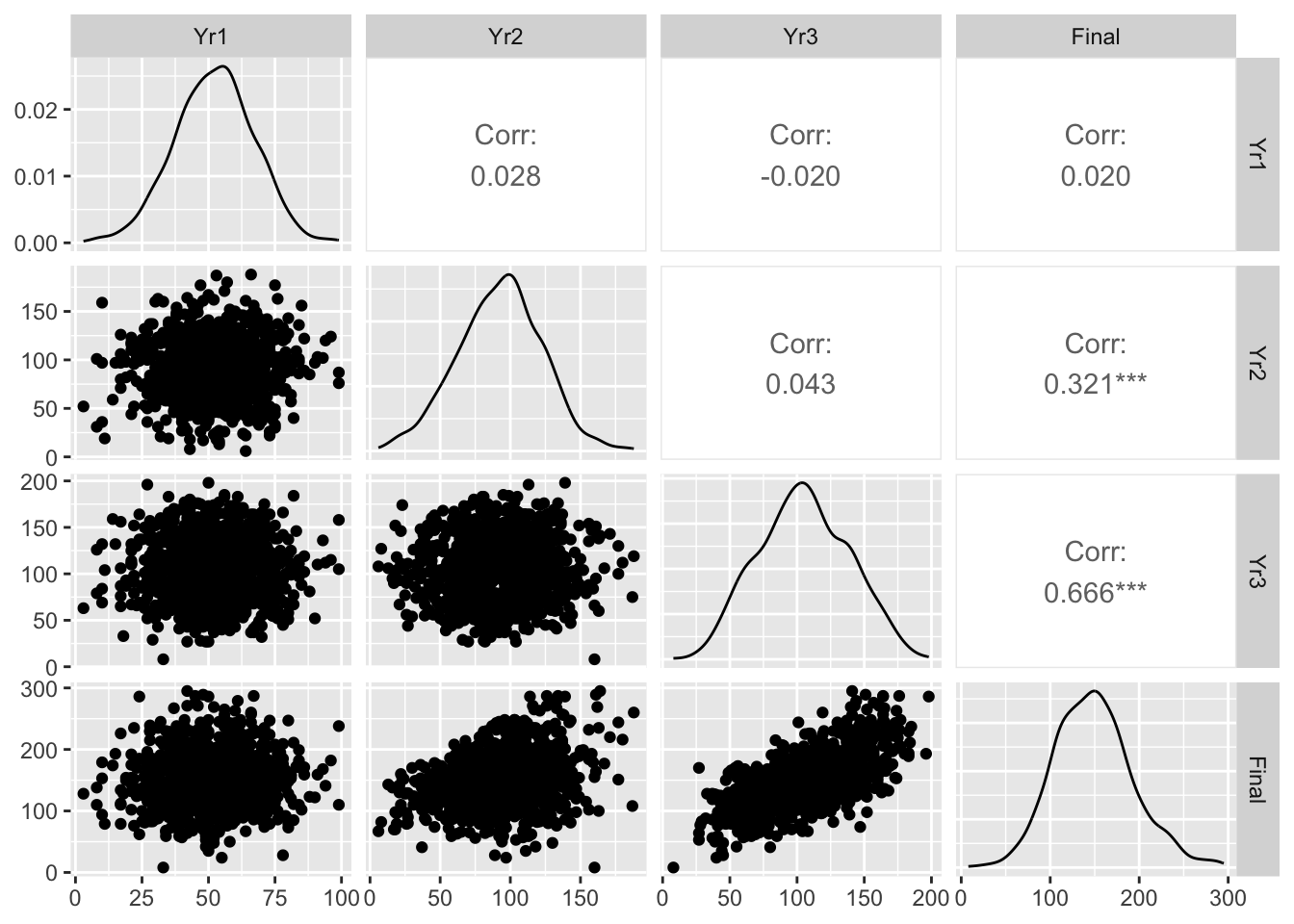
There are 975 individuals graduating in the past three years from the biology department of a large academic institution. We have data on four examinations:
a first year exam ranging from 0 to 100 (Yr1)
a second year exam ranging from 0 to 200 (Yr2)
a third year exam ranging from 0 to 200 (Yr3)
a Final year exam ranging from 0 to 300 (Final)
library (skimr); library (kableExtra); library (tidyverse)
── Attaching packages ─────────────────────────────────────── tidyverse 1.3.2 ──
✔ ggplot2 3.4.0      ✔ purrr   0.3.5
✔ tibble  3.1.8      ✔ dplyr   1.0.10
✔ tidyr   1.2.1      ✔ stringr 1.4.1
✔ readr   2.1.3      ✔ forcats 0.5.2
── Conflicts ────────────────────────────────────────── tidyverse_conflicts() ──
✖ dplyr::filter()     masks stats::filter()
✖ dplyr::group_rows() masks kableExtra::group_rows()
✖ dplyr::lag()        masks stats::lag()
skim (ugtests) %>% dplyr:: filter (skim_type== "numeric" ) %>% kable ()
skim_type
skim_variable
n_missing
complete_rate
numeric.mean
numeric.sd
numeric.p0
numeric.p25
numeric.p50
numeric.p75
numeric.p100
numeric.hist
numeric
Yr1
0
1
52.14564
14.92408
3
42
53
62
99
▁▃▇▅▁
numeric
Yr2
0
1
92.39897
30.03847
6
73
94
112
188
▁▅▇▃▁
numeric
Yr3
0
1
105.12103
33.50705
8
81
105
130
198
▁▅▇▅▁
numeric
Final
0
1
148.96205
44.33966
8
118
147
175
295
▁▅▇▃▁
A Visual of the Data
Registered S3 method overwritten by 'GGally':
  method from
  +.gg   ggplot2
# display a pairplot of all four columns of data :: ggpairs (ugtests)
<- lm (Final ~ Yr1 + Yr2 + Yr3, data= ugtests)summary (my.lm)
Call:
lm(formula = Final ~ Yr1 + Yr2 + Yr3, data = ugtests)

Residuals:
    Min      1Q  Median      3Q     Max
-92.638 -20.349   0.001  18.954  98.489

Coefficients:
            Estimate Std. Error t value Pr(>|t|)
(Intercept) 14.14599    5.48006   2.581  0.00999 **
Yr1          0.07603    0.06538   1.163  0.24519
Yr2          0.43129    0.03251  13.267  < 2e-16 ***
Yr3          0.86568    0.02914  29.710  < 2e-16 ***
---
Signif. codes:  0 '***' 0.001 '**' 0.01 '*' 0.05 '.' 0.1 ' ' 1

Residual standard error: 30.43 on 971 degrees of freedom
Multiple R-squared:  0.5303,    Adjusted R-squared:  0.5289
F-statistic: 365.5 on 3 and 971 DF,  p-value: < 2.2e-16
Basic In Sample Prediction
%>% mutate (Fitted.Value = predict (my.lm)) %>% kable () %>% scroll_box (height= "300px" )
Yr1
Yr2
Yr3
Final
Fitted.Value
27
50
52
93
82.77839
70
104
126
207
173.39734
27
36
148
175
159.84579
26
75
115
125
148.02242
46
77
75
114
115.77826
86
122
119
159
176.31713
40
100
125
153
168.52573
60
92
78
84
125.90895
49
98
119
147
163.15331
80
127
67
80
133.00197
43
134
61
154
128.01391
26
53
150
154
168.83298
64
123
110
175
167.28471
62
84
142
182
178.01432
61
65
134
155
162.81842
60
150
116
198
183.81939
58
76
107
161
143.96109
28
81
143
229
175.00126
64
87
106
100
148.29571
55
111
135
179
183.06708
77
97
111
164
157.92531
50
92
72
130
119.95460
47
83
129
194
165.18879
65
72
148
152
178.26106
57
180
112
216
193.06715
41
41
152
123
166.52931
49
90
166
232
200.39004
93
102
136
168
182.94018
32
62
160
151
181.82752
53
73
63
88
104.19713
28
84
109
184
146.86195
75
125
98
134
158.59539
44
55
111
115
137.30246
41
127
96
167
155.14171
55
97
101
170
147.59592
68
109
141
229
188.38693
73
52
124
132
149.46722
32
92
154
245
189.57199
49
65
138
180
165.36883
63
107
165
213
207.92058
43
87
120
211
158.81869
40
110
93
151
145.13679
46
71
91
121
127.04145
28
118
136
180
184.89905
46
124
176
232
223.48248
41
97
152
214
190.68129
76
95
52
123
105.91152
52
106
144
166
188.47370
47
104
124
111
169.91737
54
27
111
90
125.98673
36
97
140
187
179.91299
73
22
146
160
155.57364
60
68
54
125
94.78176
67
45
80
145
107.90209
50
99
94
168
142.01859
32
72
92
114
127.27405
75
103
91
152
143.04734
60
80
43
125
90.43469
54
13
106
143
115.62032
69
64
161
161
186.36874
54
125
107
98
164.78997
52
65
157
183
182.04486
36
138
72
152
138.72937
36
131
116
203
173.80034
39
105
116
158
162.81500
50
71
72
65
110.89761
55
110
106
133
157.53103
33
89
134
122
171.04054
52
68
135
138
164.29372
59
97
105
132
151.36275
42
101
165
174
203.73632
39
76
97
173
133.85978
45
63
131
124
158.14239
55
71
111
139
145.03931
69
55
82
119
114.09836
72
62
104
171
136.39042
61
108
98
160
150.19917
55
90
49
117
99.56150
35
84
107
178
145.66277
59
36
95
122
116.39753
44
74
87
144
124.72053
43
78
101
124
138.48918
66
142
101
244
167.84005
38
71
63
96
102.19417
62
96
147
248
187.51815
46
63
120
194
148.69592
59
105
157
198
199.82845
68
72
111
160
146.45894
54
86
79
124
123.73077
44
66
102
136
134.25546
41
87
91
127
133.56188
15
97
132
193
171.39099
52
88
107
93
148.68036
53
92
118
182
160.00402
54
71
107
114
141.50056
75
71
108
147
143.96279
52
54
98
122
126.22552
41
72
113
172
146.13759
52
74
128
108
160.82167
64
95
125
158
168.19393
64
122
78
168
139.15162
29
57
99
101
126.63646
50
107
91
163
142.87183
62
98
171
197
209.15707
45
65
134
162
161.60200
49
93
129
174
169.65369
70
37
76
137
101.21716
40
71
98
154
132.64506
50
105
81
154
133.35245
53
66
60
126
98.58109
70
110
44
105
104.99919
65
37
101
102
122.47906
79
122
69
92
132.50088
60
63
103
131
135.04371
50
114
118
189
169.26422
66
94
112
101
156.66084
46
156
135
184
201.79068
31
85
57
108
102.50589
82
99
184
211
222.36274
63
71
102
172
137.85639
33
78
78
144
117.81825
48
39
67
88
92.61602
31
80
133
153
166.14124
59
67
50
86
90.81172
60
128
94
171
155.28613
60
121
174
263
221.52163
26
108
63
158
117.23941
36
129
61
146
125.32530
63
83
115
144
154.28567
48
74
87
111
125.02463
26
132
88
81
149.23229
39
125
136
201
188.75433
46
121
113
126
167.65071
54
79
103
150
141.48812
70
95
102
136
148.73942
50
85
85
132
128.18946
34
74
144
176
173.30410
62
97
61
168
113.50085
49
56
121
141
146.77068
10
36
132
153
144.70245
50
92
99
143
143.32800
23
102
130
170
172.42426
74
126
84
110
146.83111
31
88
124
142
161.80039
38
149
86
123
155.74509
70
102
67
136
121.45958
42
104
67
111
120.19341
50
103
155
248
196.55029
56
26
90
97
107.52819
43
77
110
100
145.84903
38
83
89
106
129.87730
70
86
32
88
84.26017
50
93
103
113
147.22201
45
92
133
186
172.38103
50
123
90
146
148.90671
73
105
146
204
191.37033
59
78
47
79
92.95881
44
49
87
116
113.93839
34
58
85
59
115.32834
48
161
151
289
217.95006
53
18
96
70
109.04391
47
101
140
183
182.47442
46
149
106
189
173.66693
25
121
87
83
143.54644
71
136
156
171
213.24494
27
114
103
169
154.53040
61
106
108
110
157.99341
36
108
121
113
168.20918
66
104
91
124
142.79439
42
27
95
129
111.22351
58
116
116
174
169.00364
48
72
54
165
95.59458
80
143
137
247
200.50023
52
133
87
159
150.77458
50
37
80
41
103.15936
27
128
75
127
136.32932
44
116
98
187
152.35701
60
101
68
100
121.13371
64
97
64
150
116.24995
35
120
120
189
172.44290
34
94
56
68
105.74986
57
116
88
134
144.68854
76
163
60
100
142.16437
48
17
90
70
103.03841
74
39
55
104
84.20453
54
46
100
125
124.65866
47
70
147
168
175.16434
57
111
133
166
181.48777
56
89
146
210
183.17732
25
73
137
137
166.12881
73
26
91
79
109.68631
64
63
119
105
149.19871
67
64
118
135
148.99240
43
117
64
140
123.27911
47
123
99
154
156.46977
57
107
54
118
111.37381
21
44
114
144
133.40676
50
71
66
163
105.70352
54
116
127
144
178.22203
76
137
97
139
162.98116
48
42
61
109
88.71579
32
97
97
142
142.38459
70
57
95
116
126.29081
60
123
143
206
195.54808
76
122
57
164
121.88463
55
87
138
171
175.31327
46
89
133
183
171.16320
59
129
63
93
128.80527
64
90
115
123
157.38069
54
106
93
118
144.47601
47
106
95
164
145.67519
71
109
105
148
157.45049
54
86
41
125
90.83488
59
42
102
156
125.04501
36
111
61
73
117.56217
50
120
112
180
166.65784
57
65
111
89
142.60365
58
99
104
188
151.28361
30
73
105
110
138.80714
78
120
93
185
152.33864
36
93
139
157
177.32217
56
112
79
128
135.09624
42
111
121
172
169.95920
76
83
122
147
161.33378
65
71
117
171
150.99366
40
118
115
97
167.63206
56
59
68
105
102.71562
56
103
55
105
110.43832
81
100
111
153
159.52327
42
105
103
157
151.78922
57
124
100
174
158.52699
58
52
168
133
186.41680
27
65
93
143
124.74060
38
95
70
81
118.60478
41
98
119
155
162.54510
65
107
154
196
198.55014
60
75
84
129
123.77119
50
136
153
229
209.05134
24
114
164
286
207.10887
55
83
65
106
110.39340
73
135
71
115
139.38280
28
111
120
230
168.02915
52
105
119
167
166.40038
56
95
185
237
219.52660
38
114
90
107
144.11283
21
84
125
154
160.18067
48
92
145
172
182.99728
50
39
135
171
151.63440
50
52
129
115
152.04702
61
60
151
146
175.37858
61
123
94
162
153.20573
65
126
139
198
193.75934
42
117
86
123
142.24807
50
106
163
224
204.76959
46
49
126
132
147.85201
59
61
54
135
91.68673
62
90
140
201
178.87067
85
156
88
102
164.06869
72
131
105
152
167.01479
53
132
113
203
172.92703
21
116
67
102
123.77229
45
44
160
144
175.05272
59
95
67
101
117.60429
76
91
61
86
111.97751
53
110
109
179
159.97603
71
46
147
74
166.63812
69
110
123
138
173.31198
37
101
170
222
207.68459
50
132
76
124
140.66875
56
83
94
97
135.57418
68
100
132
181
176.71423
94
120
112
141
170.00300
37
90
132
154
170.04457
24
99
137
185
177.26620
62
68
98
135
133.02378
77
124
84
161
146.19662
29
70
139
185
166.87042
48
84
127
182
163.96474
63
124
97
127
156.38611
47
136
97
104
160.34511
50
70
27
170
71.51067
17
97
156
226
192.31939
45
92
37
128
89.27563
41
65
117
177
146.58132
79
108
84
152
139.44811
71
84
57
140
105.11565
75
30
54
170
79.53330
65
74
81
116
121.12299
52
97
58
118
110.14355
67
72
148
181
178.41312
67
38
142
135
158.55532
56
88
144
141
181.01467
61
123
152
221
203.41524
50
110
164
206
207.36041
35
81
65
90
108.01030
71
89
133
167
173.06385
52
82
107
111
146.09265
63
106
74
160
128.71230
72
97
64
135
116.85816
56
128
165
206
216.44539
64
68
140
214
169.53445
62
85
80
99
124.77337
73
114
111
182
164.95305
40
121
140
216
190.56794
57
144
56
127
129.06273
45
85
102
78
142.52591
53
25
77
128
95.61497
56
65
144
124
171.09510
27
100
149
196
188.31374
43
50
63
121
93.51730
77
80
73
166
117.69757
50
61
89
127
121.30134
47
102
135
225
178.57730
63
85
118
164
157.74528
64
161
95
164
170.68833
59
65
85
119
120.24799
49
118
55
42
116.37542
71
73
131
126
164.43192
65
106
128
146
175.61114
41
131
169
237
220.06158
71
73
151
190
181.74555
44
134
99
120
160.98583
39
56
52
95
86.27842
99
87
158
238
195.97205
17
106
87
134
136.46895
41
62
68
126
102.86908
47
119
175
231
220.53640
65
103
72
93
125.83914
57
94
147
234
186.27545
36
66
152
201
176.93132
39
103
135
159
178.40037
31
123
91
167
148.32790
44
78
151
137
181.84927
19
98
87
154
133.17072
39
119
114
157
167.12163
42
116
143
271
191.16061
33
128
111
179
167.95000
46
126
161
271
211.35983
48
125
106
154
163.46813
56
83
49
162
96.61853
60
73
117
162
151.47610
61
100
90
151
139.82344
48
109
85
164
138.38826
42
96
136
160
176.47513
54
92
56
66
106.40781
84
98
111
182
158.88878
77
126
121
195
179.08940
53
62
120
141
148.79682
58
98
95
132
143.06119
29
65
57
109
93.72813
64
82
93
114
134.88542
33
78
119
97
153.31118
55
108
60
109
116.84713
42
102
145
206
186.85398
56
140
114
178
177.47107
54
90
99
105
142.76953
65
84
125
160
163.52582
38
73
138
170
167.98283
54
92
138
155
177.39367
69
133
158
228
213.53039
55
92
119
152
161.02175
45
97
81
191
129.52203
49
139
118
201
179.97033
72
79
124
146
161.03589
57
88
93
91
136.94095
59
45
103
122
127.20454
49
109
109
226
159.24064
61
119
95
158
152.34627
58
120
136
184
188.04240
57
105
146
210
190.15391
62
114
131
227
181.43039
40
85
91
109
132.62329
56
86
129
200
167.16688
50
120
101
152
157.13535
78
133
142
209
200.36373
22
52
98
152
123.08217
34
65
59
66
95.83962
60
125
127
230
182.55975
66
77
133
138
167.50830
47
81
28
77
76.89241
45
111
87
185
140.75411
40
109
60
57
116.13802
52
97
56
132
108.41218
69
71
140
167
171.20843
48
107
52
123
108.95821
37
117
106
167
159.18156
55
73
114
152
148.49892
57
42
84
124
109.31069
28
101
92
144
139.47722
52
23
174
153
178.64745
29
110
117
110
165.07685
44
115
125
161
175.29912
65
87
116
148
157.02854
79
87
119
138
160.68996
58
104
156
159
198.45546
82
97
67
111
120.21546
58
110
95
123
148.23662
47
92
103
190
146.56264
56
81
133
182
168.47318
77
103
125
179
172.63256
28
109
157
239
199.19678
54
92
105
139
148.82619
59
81
67
114
111.56629
21
110
111
132
159.27455
47
26
56
129
77.41079
43
8
127
82
130.80692
40
92
55
111
104.47776
44
92
137
105
175.76773
49
108
95
129
146.68981
45
56
109
132
136.07840
70
134
138
191
196.72408
36
57
87
105
116.78047
60
103
52
94
108.14538
57
65
109
175
140.87229
82
40
77
85
104.28901
35
105
183
229
220.51154
37
48
100
107
124.22878
49
113
62
59
120.27876
64
87
109
162
150.89275
57
96
116
114
160.30190
24
115
69
62
125.30044
48
99
81
163
130.61268
59
89
125
174
165.22609
48
102
140
145
182.98173
39
79
169
173
197.48268
35
19
118
96
127.15171
50
77
100
108
137.72440
54
136
71
167
138.36959
63
108
143
187
189.30688
19
82
93
150
131.46424
40
117
61
134
120.45398
43
83
85
128
126.79471
69
93
116
172
159.92036
49
32
86
149
106.12099
39
84
107
94
145.96688
49
127
146
238
199.03398
61
133
144
279
200.80264
70
57
55
85
91.66356
71
84
175
219
207.26604
59
143
47
81
120.99236
72
102
82
143
134.59685
72
128
129
180
186.49729
52
46
101
147
125.37228
3
52
63
128
91.33883
56
171
143
220
215.94567
52
130
45
48
113.12211
62
132
75
109
140.71538
38
94
146
146
183.96527
49
63
75
118
109.96835
86
89
102
171
147.36813
50
107
102
167
152.39432
33
68
120
126
149.86401
17
80
65
79
106.21055
41
98
120
147
163.41078
66
141
102
178
168.27444
84
101
106
110
155.85423
32
82
98
134
136.78099
35
102
166
220
204.50110
45
65
81
137
115.72090
41
132
107
188
166.82063
80
100
58
128
113.56614
55
103
70
91
123.34751
60
105
84
151
136.70975
62
76
106
123
143.39951
25
106
85
100
135.34580
57
71
57
83
98.44458
62
104
117
212
164.99800
53
187
75
108
163.75184
71
95
113
151
158.33794
26
107
101
184
149.70401
44
99
100
106
146.75652
76
76
112
193
149.65797
42
106
160
177
201.56434
57
129
100
172
160.68342
47
94
100
153
144.82817
58
82
108
106
147.41448
50
51
85
173
113.52576
65
110
144
164
191.18718
44
136
79
145
144.53477
43
103
97
132
145.80859
64
123
85
126
145.64267
50
167
106
177
181.73417
61
60
112
106
141.61701
52
108
98
174
149.51494
75
44
108
130
132.31808
67
123
110
226
167.51278
39
53
102
129
128.26862
52
102
81
156
132.21064
48
91
43
86
94.26651
76
97
138
154
181.22267
52
65
108
169
139.62648
39
134
141
195
196.96431
39
104
80
106
131.21919
49
104
27
53
86.09835
68
90
117
135
159.41616
56
138
141
256
199.98189
61
76
77
110
118.21873
88
85
81
123
127.61573
43
96
151
198
189.53638
91
103
110
159
160.71170
26
74
70
124
108.63548
8
31
126
110
137.19988
36
79
77
116
117.61193
43
57
85
126
115.58129
54
78
150
220
181.74385
40
70
123
171
153.85581
17
71
76
110
111.85147
63
63
96
89
129.21202
67
79
86
182
127.75988
50
85
82
169
125.59242
35
139
92
183
156.39825
55
96
72
157
122.05988
65
50
104
129
130.68281
58
96
125
171
168.16906
63
89
111
198
153.41066
30
118
90
125
145.22976
33
160
8
8
92.58597
62
53
139
163
162.04743
57
133
41
76
111.33337
50
105
52
107
108.24769
46
113
117
154
167.66315
72
97
69
114
121.18656
65
123
89
207
149.18143
42
164
141
295
210.13095
54
87
147
192
183.02837
81
64
107
159
140.53427
59
120
88
149
146.56573
42
99
98
156
144.87310
47
78
133
163
166.49509
44
51
96
135
122.59210
56
60
123
153
150.75937
22
96
79
76
125.61078
55
63
47
106
86.18543
56
98
48
115
102.22212
50
102
108
135
155.43198
57
112
94
142
148.15748
62
146
78
153
149.35042
61
80
183
189
211.70608
81
89
125
157
166.89867
59
116
109
165
163.01990
41
112
116
147
165.98605
49
97
83
122
131.55750
33
59
112
111
139.05699
72
142
64
96
136.26600
38
128
133
167
187.37512
52
162
140
269
209.16296
61
100
72
134
124.24118
37
133
165
267
217.15732
71
127
66
85
131.45206
56
117
152
265
200.44739
62
97
117
157
161.97900
56
81
183
194
211.75724
50
67
173
154
196.60627
56
129
98
105
158.87603
29
137
82
146
146.42271
40
41
143
151
158.66215
63
69
53
109
94.57544
81
57
99
120
130.58982
67
156
154
232
219.83518
38
145
103
148
168.73653
52
85
56
173
103.23676
56
78
100
124
138.61184
42
74
104
164
139.28506
31
85
43
88
90.38635
50
73
67
102
107.43178
63
123
85
164
145.56665
75
177
100
151
182.75359
69
53
49
130
84.66830
42
91
45
90
95.54172
55
73
70
172
110.40895
57
95
95
151
141.69131
54
84
110
125
149.70431
57
122
98
202
155.93306
65
106
96
95
147.90934
40
27
44
80
66.92172
75
85
105
113
147.40374
53
114
112
176
164.29821
75
49
70
139
101.57863
44
117
84
144
140.66876
66
71
91
135
128.56197
52
92
142
188
180.70434
54
48
131
165
152.35734
57
54
65
86
98.03817
40
80
80
162
120.94437
66
147
94
120
163.93671
61
68
64
159
103.51459
27
113
196
193
234.60747
60
102
139
114
183.02836
49
62
79
63
112.99979
73
100
74
140
126.88485
57
48
90
175
117.09249
22
116
152
235
197.43122
34
83
158
230
189.30520
53
72
174
202
199.85646
43
96
168
201
204.25296
10
97
69
94
116.47294
29
76
97
126
133.09952
69
101
112
145
159.90792
55
97
40
24
94.78936
71
112
91
150
146.62481
47
78
127
210
161.30100
54
105
165
245
206.37377
66
60
146
208
171.43030
47
65
66
151
102.88773
74
98
55
155
109.65036
43
110
51
79
109.00625
74
78
93
170
133.92054
61
60
86
142
119.10930
59
130
68
124
133.56496
38
99
118
155
161.88262
67
126
164
287
215.55343
39
85
104
67
143.80112
54
133
72
114
137.94141
70
59
82
137
115.89952
42
96
130
154
171.28105
64
22
111
110
124.59056
44
106
72
116
125.53644
33
85
74
108
117.37452
71
91
67
96
116.79146
63
24
105
152
120.18302
42
132
43
113
111.49305
47
104
96
151
145.67830
59
85
132
191
169.56072
50
45
122
110
142.96825
71
118
149
235
199.42203
46
85
144
193
178.96055
53
106
134
140
179.89291
68
75
88
150
127.84212
42
75
137
141
168.28382
61
100
125
176
170.12228
96
124
115
182
174.47724
73
110
164
247
209.10902
69
74
115
144
150.86026
64
69
58
102
98.97987
64
116
113
116
166.86275
40
79
105
112
142.15511
55
131
96
146
157.93122
62
100
83
137
133.83970
37
86
157
192
189.96146
36
120
130
161
181.17574
36
60
86
104
117.20864
57
53
101
147
128.77141
18
103
33
128
88.50434
72
73
103
133
140.26888
11
19
104
79
113.20755
58
123
101
174
159.03742
68
83
44
108
93.20243
43
74
180
193
205.15286
10
159
84
179
156.19785
39
95
41
59
93.57605
32
96
109
108
152.34148
41
84
132
138
167.76096
47
43
87
158
111.57876
32
104
110
147
156.65744
34
84
146
133
179.34831
53
110
59
65
116.69196
61
68
103
149
137.27616
46
82
99
156
138.71104
42
72
67
89
106.39228
58
152
104
199
174.14174
79
70
100
144
136.91016
58
56
102
146
131.00698
60
78
122
137
157.96093
72
106
91
134
144.11312
63
85
109
170
149.95415
69
33
74
147
97.68463
32
21
67
142
83.63646
50
87
98
199
140.30589
43
104
141
230
184.32985
30
92
52
87
101.12046
58
84
166
186
198.48657
84
86
97
171
141.59381
58
70
85
114
122.32839
55
53
106
136
132.94777
58
83
156
155
189.39847
83
109
146
172
193.85573
44
103
91
167
140.69053
54
51
102
117
128.54644
47
81
82
123
123.63920
40
103
130
189
174.14799
42
82
27
64
76.07789
30
160
66
155
142.56740
54
139
74
110
142.26049
50
111
44
35
103.90995
69
143
84
178
153.78283
59
109
137
184
184.23997
66
72
138
140
169.68028
40
119
110
178
163.73493
53
52
130
146
153.14078
41
103
177
248
214.91104
37
121
162
222
209.38485
42
60
167
178
187.78498
65
108
144
224
190.32461
50
119
155
204
203.45085
72
76
92
151
132.04024
43
67
117
118
147.59594
45
130
157
276
209.54622
53
73
119
132
152.67528
80
97
101
73
149.49657
43
89
74
113
119.85993
29
79
125
135
158.63245
44
88
160
170
193.95325
70
139
90
141
157.32780
45
54
39
127
74.61815
49
96
93
143
139.78303
55
114
94
140
148.86800
39
95
130
232
170.62168
36
101
135
183
177.30972
59
58
113
154
141.46807
44
146
98
137
165.29557
41
45
56
102
85.14906
39
123
145
180
195.68289
54
74
51
103
94.31627
73
119
119
224
174.03493
47
88
43
114
92.89663
52
85
80
113
124.01311
61
47
158
137
175.83164
56
70
61
127
101.39999
70
79
108
106
147.03294
28
108
92
170
142.49622
47
54
71
90
102.47200
66
97
115
145
160.55174
29
105
106
153
153.39793
70
130
120
186
179.41667
71
93
118
111
161.80378
42
111
142
202
188.13850
38
130
113
158
170.92407
50
116
131
183
181.38065
49
106
138
202
183.05153
58
100
55
117
109.29652
37
105
167
206
206.81269
54
16
95
138
107.39169
64
123
90
198
149.97108
44
109
59
68
115.57644
30
85
98
155
137.92279
67
79
68
134
112.17762
52
124
104
193
161.60959
50
114
65
102
123.38311
58
46
74
121
102.45505
38
71
85
192
121.23915
28
137
84
215
148.07805
59
74
62
162
104.21889
58
113
40
89
101.91801
79
94
51
166
104.84263
57
125
101
156
159.82396
99
76
105
110
145.34680
59
110
137
218
184.67126
34
38
135
118
149.98669
54
76
177
205
204.25467
61
132
60
140
127.65413
48
60
106
152
135.43458
63
146
123
186
188.38210
53
125
45
96
111.04171
41
147
96
98
163.76741
23
78
66
124
106.66981
40
107
144
155
187.99267
30
52
152
161
170.43716
53
124
69
110
131.38677
58
137
137
211
196.23994
69
68
127
184
158.66072
32
65
84
147
117.32960
74
104
60
104
116.56648
58
69
55
131
95.92667
75
124
152
208
204.91089
14
59
159
174
178.29951
49
108
123
178
170.92889
52
55
145
149
167.34383
52
71
79
106
117.10943
53
124
110
150
166.87970
61
100
131
170
175.31637
38
154
79
115
151.84175
62
84
91
116
133.86458
45
109
96
151
147.68267
21
123
132
192
183.06057
37
90
97
110
139.74572
75
121
138
171
191.49750
52
62
130
130
157.37761
31
163
138
235
206.26633
55
97
116
101
160.58114
47
85
155
201
188.55907
57
110
103
149
155.08604
61
100
111
187
158.00274
50
94
128
120
169.29532
40
104
79
110
130.42954
71
57
85
111
117.71002
50
119
48
82
110.82296
54
78
74
99
115.95208
36
112
77
118
131.84435
32
117
108
191
160.53279
61
75
123
145
157.60878
38
55
112
136
137.71198
58
90
173
243
207.13405
31
93
63
152
111.15026
60
117
75
120
134.09404
34
95
155
190
191.88358
44
112
90
206
143.70642
63
102
138
198
182.39076
59
46
98
139
123.30742
35
96
89
113
135.25593
60
96
115
114
159.66430
53
89
94
108
137.93381
57
144
79
163
148.97340
39
46
103
145
126.11531
43
75
54
109
96.50831
46
109
67
121
122.65395
33
118
108
114
161.04010
35
62
161
173
182.92128
56
57
84
186
115.70395
65
87
78
134
124.13266
49
36
112
143
130.35385
38
84
63
141
107.80088
46
58
77
99
109.31520
75
69
116
141
150.02567
43
138
102
167
165.23199
90
97
52
122
107.83846
60
112
164
243
208.98325
32
124
140
213
191.25359
71
83
89
162
132.38617
57
121
72
124
132.99406
58
139
53
86
124.38528
66
118
139
174
190.38509
53
81
133
151
168.24510
64
42
124
111
144.47013
59
110
139
179
186.40262
62
132
136
242
193.52193
49
111
154
218
199.05886
70
60
166
165
189.04803
56
124
108
148
165.37642
45
134
176
287
227.71931
69
87
144
182
181.57172
56
105
151
164
194.40629
68
42
89
128
114.47539
68
97
76
111
126.94223
44
123
119
212
173.55531
33
87
138
208
173.64069
66
81
37
119
86.12804
44
149
89
154
158.79830
68
116
104
131
159.37572
56
77
73
89
114.80716
8
101
79
138
126.70284
74
100
81
126
133.02065
47
107
78
129
131.38989
29
66
29
83
69.92034
68
96
84
108
133.43639
46
100
63
100
115.30965
49
103
130
150
174.83223
43
77
77
106
117.28155
68
149
152
190
215.16084
64
6
108
67
115.09295
49
57
88
140
118.63449
72
125
88
155
149.71050
56
48
69
119
98.83716
39
59
110
173
137.78178
48
94
114
189
157.02373
70
92
141
203
181.20713
46
90
105
170
147.35541
57
65
103
151
135.67820
62
92
120
169
162.41962
62
64
88
129
122.64183
55
64
139
94
166.25939
45
132
105
205
165.39337
37
125
118
165
173.02002
46
39
125
132
142.67348
31
75
80
88
118.10370
61
59
89
142
121.27506
43
18
152
98
156.76180
67
110
41
98
102.17407
54
83
67
69
112.04873
17
126
106
112
161.54260
64
46
124
162
146.19527
49
92
109
154
151.90878
47
55
66
153
98.57488
61
75
113
159
148.95197
27
114
88
116
141.54518
52
79
107
118
144.79879
22
96
91
138
135.99896
66
137
164
257
220.22154
31
122
113
170
166.94160
42
53
151
135
170.91508
57
86
91
128
134.34702
60
41
120
128
140.27201
50
61
121
192
149.00314
68
137
119
175
181.41794
58
70
159
159
186.38880
39
64
78
134
112.23641
58
84
95
142
137.02320
72
124
89
136
150.14489
40
104
106
225
153.80293
43
43
113
148
133.78237
66
93
136
178
177.00591
53
59
62
87
97.29345
49
124
123
161
177.82945
70
65
71
101
108.96474
50
83
104
141
143.77484
59
47
82
141
109.88781
54
99
89
125
137.99429
52
80
165
136
195.43959
42
86
91
148
133.20663
58
115
112
147
165.10963
44
78
55
119
98.74387
80
89
51
85
102.76223
62
103
139
220
183.61170
50
139
198
286
249.30085
50
106
133
192
178.79915
50
141
79
127
147.14736
52
75
37
56
82.47596
63
80
171
176
201.46996
66
45
130
139
151.11012
50
104
83
141
134.65252
58
94
39
50
92.85790
53
50
96
169
122.84505
45
94
94
115
139.48203
35
137
120
183
179.77475
43
100
128
174
171.35085
38
101
131
238
173.99905
44
158
147
193
212.88938
56
90
79
81
125.60796
37
46
163
130
177.90413
47
97
122
167
165.16701
70
102
119
150
166.47500
50
92
66
59
114.76052
45
116
79
130
135.98509
53
21
93
130
107.74073
41
75
137
203
168.20780
49
110
164
182
207.28439
64
60
97
111
128.85987
67
129
114
183
173.56322
72
46
99
178
125.16145
67
96
37
86
92.67335
47
78
128
158
162.16668
47
177
130
244
206.59530
54
89
151
172
187.35367
56
64
137
125
164.60405
34
123
104
134
159.80983
57
81
87
98
128.72787
59
134
107
169
169.05167
75
33
110
118
129.30531
28
114
56
83
113.91941
31
31
100
122
116.44077
55
108
95
181
147.14597
41
31
99
124
116.33535
48
106
156
215
198.55777
40
36
119
109
135.72938
21
118
110
175
161.85915
38
147
102
136
168.73342
34
122
111
183
165.43831
62
94
62
150
113.07268
71
81
137
213
173.07630
78
89
45
28
97.41609
36
93
123
207
163.47127
31
123
108
176
163.04448
84
136
115
199
178.74035
34
119
108
166
161.54741
41
80
68
142
110.63222
45
86
151
125
185.37558
46
94
112
171
155.14032
55
58
44
92
81.43196
64
115
61
97
121.41604
48
98
125
154
168.27137
54
80
74
136
116.81465
66
81
125
99
162.30799
56
44
105
110
128.27654
46
110
135
223
181.95155
49
56
74
72
106.08367
66
188
119
260
203.26144
41
89
79
123
124.03628
50
75
159
154
187.93702
64
139
92
165
158.60301
46
55
47
150
82.05091
49
129
109
166
167.86634
78
68
166
176
193.10652
44
61
116
155
144.21857
80
97
121
148
166.81020
37
79
120
178
154.91225
58
135
125
172
184.98919
Out of Sample Prediction
Suppose we have a student with a 55 on Yr1, a 95 on Yr2 and a 110 on Yr3.
First, what would their data look like?
<- data.frame (Yr1= 55 , Yr2= 95 , Yr3= 110 )
Let’s predict, first the single best guess – the fitted value.
The equation we sought estimates for was:
library (equatiomatic):: extract_eq (my.lm)
\[
\operatorname{Final} = \alpha + \beta_{1}(\operatorname{Yr1}) + \beta_{2}(\operatorname{Yr2}) + \beta_{3}(\operatorname{Yr3}) + \epsilon
\]
And it was estimated to be
:: extract_eq (my.lm, use_coefs = TRUE , coef_digits = 4 )
\[
\operatorname{\widehat{Final}} = 14.146 + 0.076(\operatorname{Yr1}) + 0.4313(\operatorname{Yr2}) + 0.8657(\operatorname{Yr3})
\]
Our best guess for Hypothetical.Student must then be:
14.145 + 0.076 * 55 + 0.4313 * 95 + 0.8657 * 110
What does predict produce?
predict (my.lm, newdata = Hypothetical.Student)
The same thing except that mine by hand was restricted to four digits.
In exact form, we could produce, using matrix multiplication,
c (summary (my.lm)$ coefficients[,1 ])
(Intercept) Yr1 Yr2 Yr3
14.14598945 0.07602621 0.43128539 0.86568123
c (1 ,Hypothetical.Student)
[[1]]
[1] 1
$Yr1
[1] 55
$Yr2
[1] 95
$Yr3
[1] 110
c (1 ,55 ,95 ,110 )%*% c (summary (my.lm)$ coefficients[,1 ])
Because that is all predict does.
Confidence Interval
To produce confidence intervals, we can add the interval option. For an interval of the predicted average, we have:
predict (my.lm, newdata = Hypothetical.Student, interval= "confidence" )
fit lwr upr
1 154.5245 152.551 156.498
Prediction Interval
An interval of the predicted range of data, we have
predict (my.lm, newdata = Hypothetical.Student, interval= "prediction" )
fit lwr upr
1 154.5245 94.76778 214.2812
Smart Prediction
One great thing about R is smart prediction . So what does it do? Let’s try out the centering operations that I used.
<- lm (Final ~ scale (Yr1, scale= FALSE ) + scale (Yr2, scale= FALSE ) + scale (Yr3, scale= FALSE ), data= ugtests)summary (my.lm)
Call:
lm(formula = Final ~ scale(Yr1, scale = FALSE) + scale(Yr2, scale = FALSE) +
scale(Yr3, scale = FALSE), data = ugtests)
Residuals:
Min 1Q Median 3Q Max
-92.638 -20.349 0.001 18.954 98.489
Coefficients:
Estimate Std. Error t value Pr(>|t|)
(Intercept) 148.96205 0.97467 152.833 <2e-16 ***
scale(Yr1, scale = FALSE) 0.07603 0.06538 1.163 0.245
scale(Yr2, scale = FALSE) 0.43129 0.03251 13.267 <2e-16 ***
scale(Yr3, scale = FALSE) 0.86568 0.02914 29.710 <2e-16 ***
---
Signif. codes: 0 '***' 0.001 '**' 0.01 '*' 0.05 '.' 0.1 ' ' 1
Residual standard error: 30.43 on 971 degrees of freedom
Multiple R-squared: 0.5303, Adjusted R-squared: 0.5289
F-statistic: 365.5 on 3 and 971 DF, p-value: < 2.2e-16
:: extract_eq (my.lm, use_coefs = TRUE , coef_digits = 4 )
\[
\operatorname{\widehat{Final}} = 148.9621 + 0.076(\operatorname{scale(Yr1,\ scale\ =\ FALSE)}) + 0.4313(\operatorname{scale(Yr2,\ scale\ =\ FALSE)}) + 0.8657(\operatorname{scale(Yr3,\ scale\ =\ FALSE)})
\]
Only the intercept is impacted; the original intercept was the expected Final for a student that had all zeroes [possible but a very poor performance] and they’d have expected a 14.15 [the original intercept]. After the centering operation for each predictor, the average student [mean scores on Yr1, Yr2, and Yr3] could expect a score of 148.96205 – the intercept from the regression on centered data.
Now let’s predict our Hypothetical.Student.
predict (my.lm, newdata= Hypothetical.Student)
The result is the same.
predict (my.lm, newdata= Hypothetical.Student, interval= "confidence" )
       fit     lwr     upr
1 154.5245 152.551 156.498
predict (my.lm, newdata= Hypothetical.Student, interval= "prediction" )
       fit      lwr      upr
1 154.5245 94.76778 214.2812
This works because R knows that each variable was centered, the mean was subtracted because that is what scale does when the [unfortunately named] argument scale inside the function scale is set to FALSE => we are not creating z-scores [the default is \(\frac{x_{i} - \overline{x}}{sd(x)}\) ] but are just taking \(x_{i} - \overline{x}\) or centering the data .
Smart Prediction is Deployed Throughout R
Let me try a regression where Yr1, Yr2, and Yr3 are allowed to have effects with curvature using each term and its square.
<- lm (Final ~ Yr1 + Yr1^ 2 + Yr2 + Yr2^ 2 + Yr3 + Yr3^ 2 , data= ugtests)summary (my.lm.Sq)
Call:
lm(formula = Final ~ Yr1 + Yr1^2 + Yr2 + Yr2^2 + Yr3 + Yr3^2,
    data = ugtests)

Residuals:
    Min      1Q  Median      3Q     Max
-92.638 -20.349   0.001  18.954  98.489

Coefficients:
            Estimate Std. Error t value Pr(>|t|)
(Intercept) 14.14599    5.48006   2.581  0.00999 **
Yr1          0.07603    0.06538   1.163  0.24519
Yr2          0.43129    0.03251  13.267  < 2e-16 ***
Yr3          0.86568    0.02914  29.710  < 2e-16 ***
---
Signif. codes:  0 '***' 0.001 '**' 0.01 '*' 0.05 '.' 0.1 ' ' 1

Residual standard error: 30.43 on 971 degrees of freedom
Multiple R-squared:  0.5303,    Adjusted R-squared:  0.5289
F-statistic: 365.5 on 3 and 971 DF,  p-value: < 2.2e-16
Unfortunately, that did not actually include the squared terms, we still only have three lines. We could use this:
<- lm (Final ~ Yr1 + Yr1* Yr1 + Yr2 + Yr2* Yr2 + Yr3 + Yr3* Yr3, data= ugtests)summary (my.lm.Sq)
Call:
lm(formula = Final ~ Yr1 + Yr1 * Yr1 + Yr2 + Yr2 * Yr2 + Yr3 +
    Yr3 * Yr3, data = ugtests)

Residuals:
    Min      1Q  Median      3Q     Max
-92.638 -20.349   0.001  18.954  98.489

Coefficients:
            Estimate Std. Error t value Pr(>|t|)
(Intercept) 14.14599    5.48006   2.581  0.00999 **
Yr1          0.07603    0.06538   1.163  0.24519
Yr2          0.43129    0.03251  13.267  < 2e-16 ***
Yr3          0.86568    0.02914  29.710  < 2e-16 ***
---
Signif. codes:  0 '***' 0.001 '**' 0.01 '*' 0.05 '.' 0.1 ' ' 1

Residual standard error: 30.43 on 971 degrees of freedom
Multiple R-squared:  0.5303,    Adjusted R-squared:  0.5289
F-statistic: 365.5 on 3 and 971 DF,  p-value: < 2.2e-16
But that also does not work. The key is to give \(R\) an object for the squared term that treats Yr1, Yr2, and Yr3 as base terms to be squared; the function for this is I.
<- lm (Final ~ Yr1 + I (Yr1^ 2 ) + Yr2 + I (Yr2^ 2 ) + Yr3 + I (Yr3^ 2 ), data= ugtests)summary (my.lm.Sq)
Call:
lm(formula = Final ~ Yr1 + I(Yr1^2) + Yr2 + I(Yr2^2) + Yr3 +
    I(Yr3^2), data = ugtests)

Residuals:
    Min      1Q  Median      3Q     Max
-94.292 -19.764  -0.006  18.961  93.503

Coefficients:
              Estimate Std. Error t value Pr(>|t|)
(Intercept) 24.4243935 13.4033492   1.822   0.0687 .
Yr1          0.2023539  0.3209042   0.631   0.5285
I(Yr1^2)    -0.0011955  0.0030483  -0.392   0.6950
Yr2          0.3434989  0.1446076   2.375   0.0177 *
I(Yr2^2)     0.0004756  0.0007687   0.619   0.5362
Yr3          0.6617121  0.1549276   4.271 2.14e-05 ***
I(Yr3^2)     0.0009624  0.0007183   1.340   0.1806
---
Signif. codes:  0 '***' 0.001 '**' 0.01 '*' 0.05 '.' 0.1 ' ' 1

Residual standard error: 30.45 on 968 degrees of freedom
Multiple R-squared:  0.5314,    Adjusted R-squared:  0.5285
F-statistic:   183 on 6 and 968 DF,  p-value: < 2.2e-16
Does the curvature improve fit? We can use an F test.
Analysis of Variance Table

Model 1: Final ~ scale(Yr1, scale = FALSE) + scale(Yr2, scale = FALSE) +
    scale(Yr3, scale = FALSE)
Model 2: Final ~ Yr1 + I(Yr1^2) + Yr2 + I(Yr2^2) + Yr3 + I(Yr3^2)
  Res.Df    RSS Df Sum of Sq      F Pr(>F)
1    971 899371
2    968 897272  3    2098.6 0.7547 0.5197
We cannot tell the two models apart so the squared terms do not improve the model. That wasn’t really the goal, it was to illustrate Smart Prediction.
What would we expect, given this new model, for our hypothetical student?
predict (my.lm.Sq, newdata= Hypothetical.Student)
I will forego the intervals but it just works because R knows to square each of Yr1, Yr2, and Yr3.
An Interaction Term
Suppose that Yr1 and Yr2 have an interactive effect. We could use the I() construct but we do not have to. The regression would be:
<- lm (Final ~ Yr1 + Yr2 + Yr1* Yr2 + Yr3, data= ugtests)summary (my.lm.Int)
Call:
lm(formula = Final ~ Yr1 + Yr2 + Yr1 * Yr2 + Yr3, data = ugtests)

Residuals:
    Min      1Q  Median      3Q     Max
-94.745 -20.774  -0.013  19.112  98.618

Coefficients:
             Estimate Std. Error t value Pr(>|t|)
(Intercept)  2.961723  11.930732   0.248    0.804
Yr1          0.290161   0.213180   1.361    0.174
Yr2          0.550808   0.117829   4.675 3.36e-06 ***
Yr3          0.866264   0.029141  29.727  < 2e-16 ***
Yr1:Yr2     -0.002295   0.002175  -1.055    0.292
---
Signif. codes:  0 '***' 0.001 '**' 0.01 '*' 0.05 '.' 0.1 ' ' 1

Residual standard error: 30.43 on 970 degrees of freedom
Multiple R-squared:  0.5309,    Adjusted R-squared:  0.5289
F-statistic: 274.4 on 4 and 970 DF,  p-value: < 2.2e-16
<- lm (Final ~ Yr1 + Yr2 + I (Yr1* Yr2) + Yr3, data= ugtests)summary (my.lm.I)
Call:
lm(formula = Final ~ Yr1 + Yr2 + I(Yr1 * Yr2) + Yr3, data = ugtests)

Residuals:
    Min      1Q  Median      3Q     Max
-94.745 -20.774  -0.013  19.112  98.618

Coefficients:
              Estimate Std. Error t value Pr(>|t|)
(Intercept)   2.961723  11.930732   0.248    0.804
Yr1           0.290161   0.213180   1.361    0.174
Yr2           0.550808   0.117829   4.675 3.36e-06 ***
I(Yr1 * Yr2) -0.002295   0.002175  -1.055    0.292
Yr3           0.866264   0.029141  29.727  < 2e-16 ***
---
Signif. codes:  0 '***' 0.001 '**' 0.01 '*' 0.05 '.' 0.1 ' ' 1

Residual standard error: 30.43 on 970 degrees of freedom
Multiple R-squared:  0.5309,    Adjusted R-squared:  0.5289
F-statistic: 274.4 on 4 and 970 DF,  p-value: < 2.2e-16
It is worth noting that this does not improve the fit of the model.
Analysis of Variance Table

Model 1: Final ~ scale(Yr1, scale = FALSE) + scale(Yr2, scale = FALSE) +
    scale(Yr3, scale = FALSE)
Model 2: Final ~ Yr1 + Yr2 + I(Yr1 * Yr2) + Yr3
  Res.Df    RSS Df Sum of Sq      F Pr(>F)
1    971 899371
2    970 898340  1    1031.5 1.1137 0.2915
Analysis of Variance Table

Model 1: Final ~ scale(Yr1, scale = FALSE) + scale(Yr2, scale = FALSE) +
    scale(Yr3, scale = FALSE)
Model 2: Final ~ Yr1 + Yr2 + Yr1 * Yr2 + Yr3
  Res.Df    RSS Df Sum of Sq      F Pr(>F)
1    971 899371
2    970 898340  1    1031.5 1.1137 0.2915
The same holds for both:
predict (my.lm.I, newdata= Hypothetical.Student)predict (my.lm.Int, newdata= Hypothetical.Student)
An Addendum on Diagnosing Quadratics
Let me generate some fake data to showcase use cases for quadratic functions of x as determinants of y.
The True Model
I will generate \(y\) according to the following equation.
\[y = x + 2*x^2 + \epsilon\]
where x is a sequence from -5 to 5 and \(\epsilon\) is Normal(0,1).
Attaching package: 'magrittr'
The following object is masked from 'package:purrr':

    set_names
The following object is masked from 'package:tidyr':

    extract
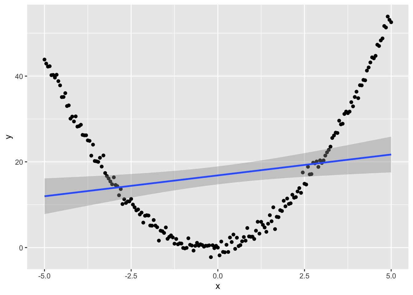
<- data.frame (x= seq (- 5 ,5 , by= 0.05 ))$ y <- fake.df$ x + 2 * fake.df$ x^ 2 + rnorm (201 )
A Plot
Let me plot x and y and include the estimated regression line [that does not include the squared term].
%>% ggplot () + aes (x= x, y= y) + geom_point () + geom_smooth (method= "lm" )
`geom_smooth()` using formula = 'y ~ x'
To be transparent, here is the regression.
summary (lm (y~ x, data= fake.df))
Call:
lm(formula = y ~ x, data = fake.df)

Residuals:
    Min      1Q  Median      3Q     Max
-18.881 -13.564  -4.011  11.655  32.283

Coefficients:
            Estimate Std. Error t value Pr(>|t|)
(Intercept)  16.8459     1.0606  15.884  < 2e-16 ***
x             0.9736     0.3656   2.663  0.00837 **
---
Signif. codes:  0 '***' 0.001 '**' 0.01 '*' 0.05 '.' 0.1 ' ' 1

Residual standard error: 15.04 on 199 degrees of freedom
Multiple R-squared:  0.03441,   Adjusted R-squared:  0.02956
F-statistic: 7.093 on 1 and 199 DF,  p-value: 0.008374
Note just looking at the table would suggest we conclude that \(y\) is a linear function of \(x\) and this is, at best, partially true. It is actually a quadratic function of \(x\) . The fit is not very good, though.
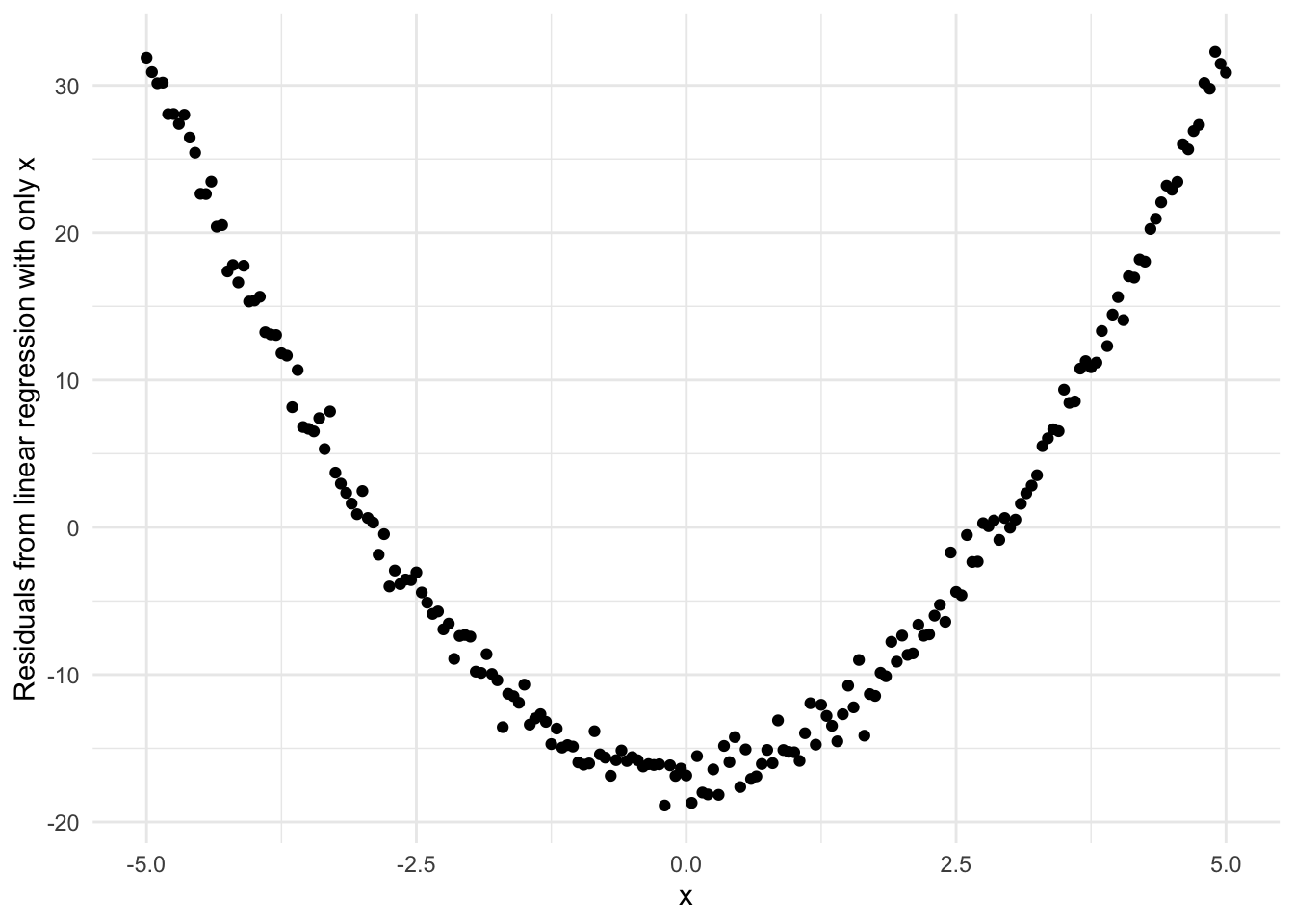
What do the residuals look like?
%<>% mutate (resid = lm (y~ x, fake.df)$ residuals)%>% ggplot () + aes (x= x, y= resid) + geom_point () + theme_minimal () + labs (y= "Residuals from linear regression with only x" )
This is a characteristic pattern of a quadratic, a because the inflection point is at zero and \(x\) can be both positive or negative. Real world data is almost always a bit messier. Nevertheless, I digress. Let’s look at the regression estimates including a squared term.
summary (lm (y~ x+ I (x^ 2 ), fake.df))
Call:
lm(formula = y ~ x + I(x^2), data = fake.df)

Residuals:
     Min       1Q   Median       3Q      Max
-2.85154 -0.72408 -0.00959  0.55789  3.07849

Coefficients:
            Estimate Std. Error t value Pr(>|t|)
(Intercept) 0.158945   0.111171    1.43    0.154
x           0.973576   0.025546   38.11   <2e-16 ***
I(x^2)      1.982605   0.009845  201.38   <2e-16 ***
---
Signif. codes:  0 '***' 0.001 '**' 0.01 '*' 0.05 '.' 0.1 ' ' 1

Residual standard error: 1.051 on 198 degrees of freedom
Multiple R-squared:  0.9953,    Adjusted R-squared:  0.9953
F-statistic: 2.1e+04 on 2 and 198 DF,  p-value: < 2.2e-16
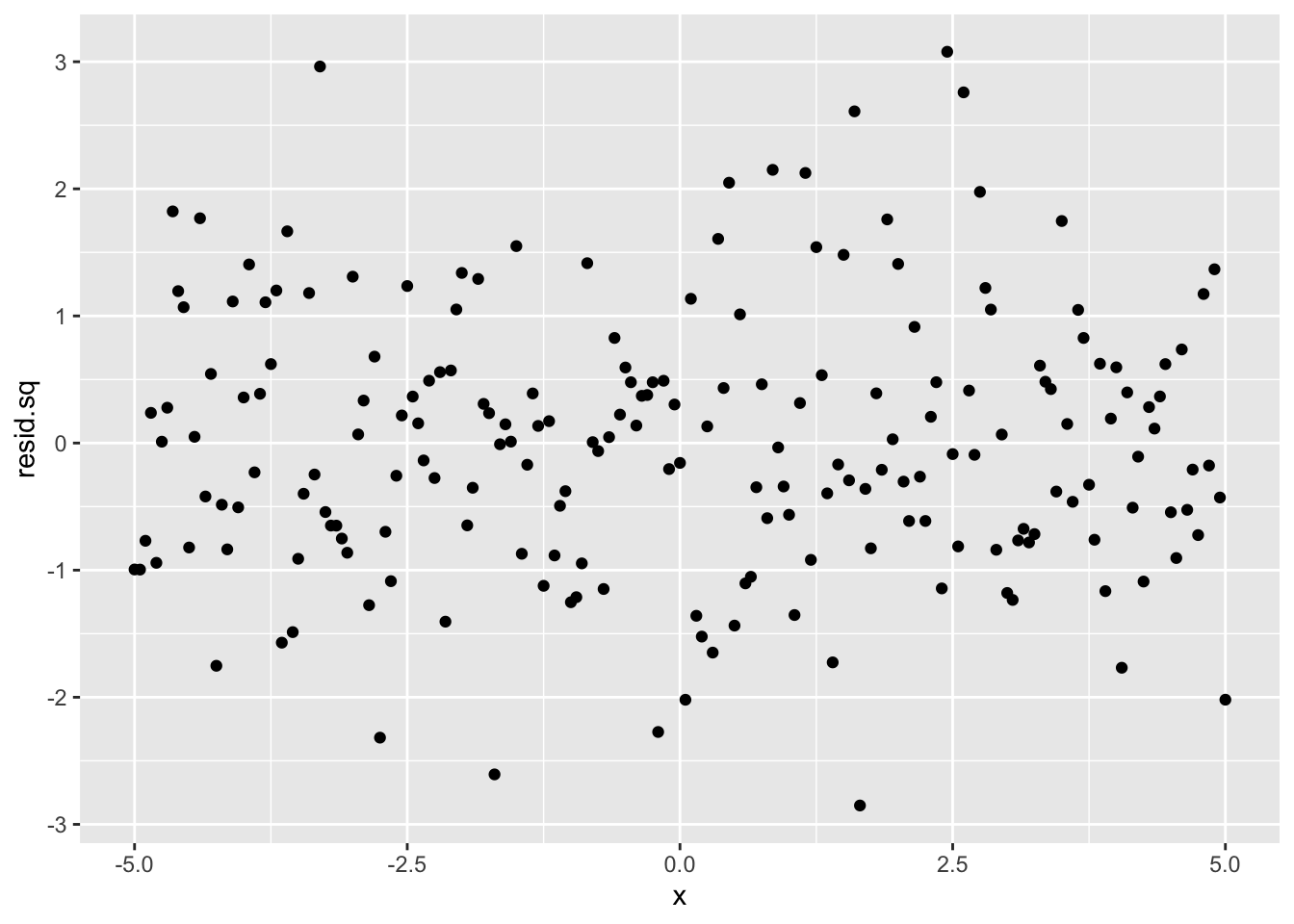
Notice both the linear and the squared term are statistically different from zero and that the linear term has a much smaller standard error because it is far more precisely estimated. What do the residuals now look like?
%<>% mutate (resid.sq = lm (y~ x+ I (x^ 2 ), fake.df)$ residuals)%>% ggplot () + aes (x= x, y= resid.sq) + geom_point ()
These are basically random with respect to \(x\) .
I should also point out that the residuals are well behaved now; they were not in the previous case.
library (gvlma)gvlma (lm (y~ x, data= fake.df))
Call:
lm(formula = y ~ x, data = fake.df)

Coefficients:
(Intercept)            x
    16.8459       0.9736


ASSESSMENT OF THE LINEAR MODEL ASSUMPTIONS
USING THE GLOBAL TEST ON 4 DEGREES-OF-FREEDOM:
Level of Significance =  0.05

Call:
 gvlma(x = lm(y ~ x, data = fake.df))

                       Value   p-value                   Decision
Global Stat        2.193e+02 0.0000000 Assumptions NOT satisfied!
Skewness           1.275e+01 0.0003564 Assumptions NOT satisfied!
Kurtosis           6.495e+00 0.0108195 Assumptions NOT satisfied!
Link Function      2.000e+02 0.0000000 Assumptions NOT satisfied!
Heteroscedasticity 7.628e-03 0.9304026    Assumptions acceptable.
Versus
gvlma (lm (y~ x+ I (x^ 2 ), data= fake.df))
Call:
lm(formula = y ~ x + I(x^2), data = fake.df)

Coefficients:
(Intercept)            x       I(x^2)
     0.1589       0.9736       1.9826


ASSESSMENT OF THE LINEAR MODEL ASSUMPTIONS
USING THE GLOBAL TEST ON 4 DEGREES-OF-FREEDOM:
Level of Significance =  0.05

Call:
 gvlma(x = lm(y ~ x + I(x^2), data = fake.df))

                       Value p-value                Decision
Global Stat        4.7545761  0.3134 Assumptions acceptable.
Skewness           1.8889919  0.1693 Assumptions acceptable.
Kurtosis           0.5404830  0.4622 Assumptions acceptable.
Link Function      2.3249033  0.1273 Assumptions acceptable.
Heteroscedasticity 0.0001979  0.9888 Assumptions acceptable.