tidyTuesday: coffee chains

The tidyTuesday for this week is coffee chain locations

For this week: 1. The basic link to the #tidyTuesday shows an original article for Week 6.

The page notes that Starbucks, Tim Horton, and Dunkin Donuts have raw data available. The data come in Excel format. We will first need to import them from Excel and then manipulate it. You can find the file in the github repository here

Code

library(readxl)
library(tidyverse)
library(janitor)
library(geofacet)
library(ggbeeswarm)
library(ggrepel)
library(leaflet)
Starbucks <- read_excel("data/coffee.xlsx", sheet = "starbucks")
Dunkin.Donuts <- read_excel("data/coffee.xlsx", 
    sheet = "dunkin", col_types = c("numeric", 
        "text", "text", "text", "text", "text", 
        "text", "text", "text", "numeric", 
        "numeric", "numeric", "text", "text", 
        "text", "numeric", "numeric", "numeric", 
        "numeric", "text", "text", "text"))
Tim.Hortons <- read_excel("data/coffee.xlsx", 
    sheet = "timhorton")

What do the data look like?

Starbucks Data

Code

library(skimr)
Starbucks <- Starbucks %>% mutate(popup = paste0(`Store Name`,"<br>",`Street Address`, "<br>", City, ", ", `State/Province`,"<br>",Postcode,"<br>",Country, sep=""))
skim(Starbucks)

Data summary

Name	Starbucks
Number of rows	25600
Number of columns	14
_______________________
Column type frequency:
character	12
numeric	2
________________________
Group variables	None

Variable type: character

skim_variable	n_missing	complete_rate	min	max	empty	n_unique	whitespace
Brand	0	1.00	7	21	0	4	0
Store Number	0	1.00	5	12	0	25599	0
Store Name	0	1.00	2	60	0	25364	0
Ownership Type	0	1.00	8	13	0	4	0
Street Address	2	1.00	1	234	0	25353	0
City	14	1.00	2	29	0	5470	0
State/Province	0	1.00	1	3	0	338	0
Country	0	1.00	2	2	0	73	0
Postcode	1521	0.94	1	9	0	18888	0
Phone Number	6861	0.73	1	18	0	18559	0
Timezone	0	1.00	18	30	0	101	0
popup	0	1.00	42	310	0	25597	0

Variable type: numeric

skim_variable	n_missing	complete_rate	mean	sd	p0	p25	p50	p75	p100	hist
Longitude	1	1	-27.87	96.84	-159.46	-104.66	-79.35	100.63	176.92	▇▇▂▂▅
Latitude	1	1	34.79	13.34	-46.41	31.24	36.75	41.57	64.85	▁▁▁▇▂

Dunkin Donuts Data

Code

skim(Dunkin.Donuts)

Data summary

Name	Dunkin.Donuts
Number of rows	4898
Number of columns	22
_______________________
Column type frequency:
character	14
numeric	8
________________________
Group variables	None

Variable type: character

skim_variable	n_missing	complete_rate	min	max	empty	n_unique	whitespace
biz_name	0	1.00	8	38	0	33	0
e_address	0	1.00	6	61	0	4864	0
e_city	0	1.00	2	27	0	1770	0
e_state	0	1.00	2	2	0	41	0
e_postal	0	1.00	4	5	0	2554	0
e_zip_full	0	1.00	10	10	0	545	0
e_country	0	1.00	3	3	0	1	0
loc_county	0	1.00	3	21	0	395	0
loc_PMSA	0	1.00	2	4	0	53	0
loc_TZ	0	1.00	3	5	0	5	0
loc_DST	0	1.00	1	1	0	3	0
web_url	0	1.00	20	175	0	22	0
biz_info	4091	0.16	14	18	0	709	0
biz_phone	0	1.00	14	14	0	4562	0

Variable type: numeric

skim_variable	n_missing	complete_rate	mean	sd	p0	p25	p50	p75	p100	hist
id	0	1	2459.46	1420.28	1.00	1231.25	2458.50	3686.75	4920.00	▇▇▇▇▇
loc_area_code	0	1	590.09	229.26	201.00	401.00	610.00	781.00	989.00	▇▅▇▇▆
loc_FIPS	0	1	27911.17	12470.14	1069.00	17031.00	26125.00	36111.00	55111.00	▂▅▆▇▂
loc_MSA	0	1	4284.65	2849.57	160.00	1520.00	3800.00	6880.00	9320.00	▇▃▂▆▅
loc_LAT_centroid	0	1	39.62	4.33	21.42	39.39	41.22	42.11	47.63	▁▁▁▇▂
loc_LAT_poly	0	1	39.62	4.32	21.39	39.38	41.20	42.09	47.64	▁▁▁▇▂
loc_LONG_centroid	0	1	-77.55	7.31	-157.93	-81.44	-75.08	-72.66	-67.23	▁▁▁▁▇
loc_LONG_poly	0	1	-77.55	7.31	-157.96	-81.44	-75.08	-72.66	-67.28	▁▁▁▁▇

Tim Horton’s Data

Code

skim(Tim.Hortons)

Data summary

Name	Tim.Hortons
Number of rows	4955
Number of columns	6
_______________________
Column type frequency:
character	6
________________________
Group variables	None

Variable type: character

skim_variable	n_missing	complete_rate	min	max	empty	n_unique	whitespace
country	0	1	2	2	0	2	0
address	0	1	6	51	0	4803	0
city	0	1	3	38	0	1206	0
postal_code	0	1	4	7	0	4328	0
state	0	1	2	2	0	27	0
store_name	0	1	2	63	0	3167	0

Plot Starbucks

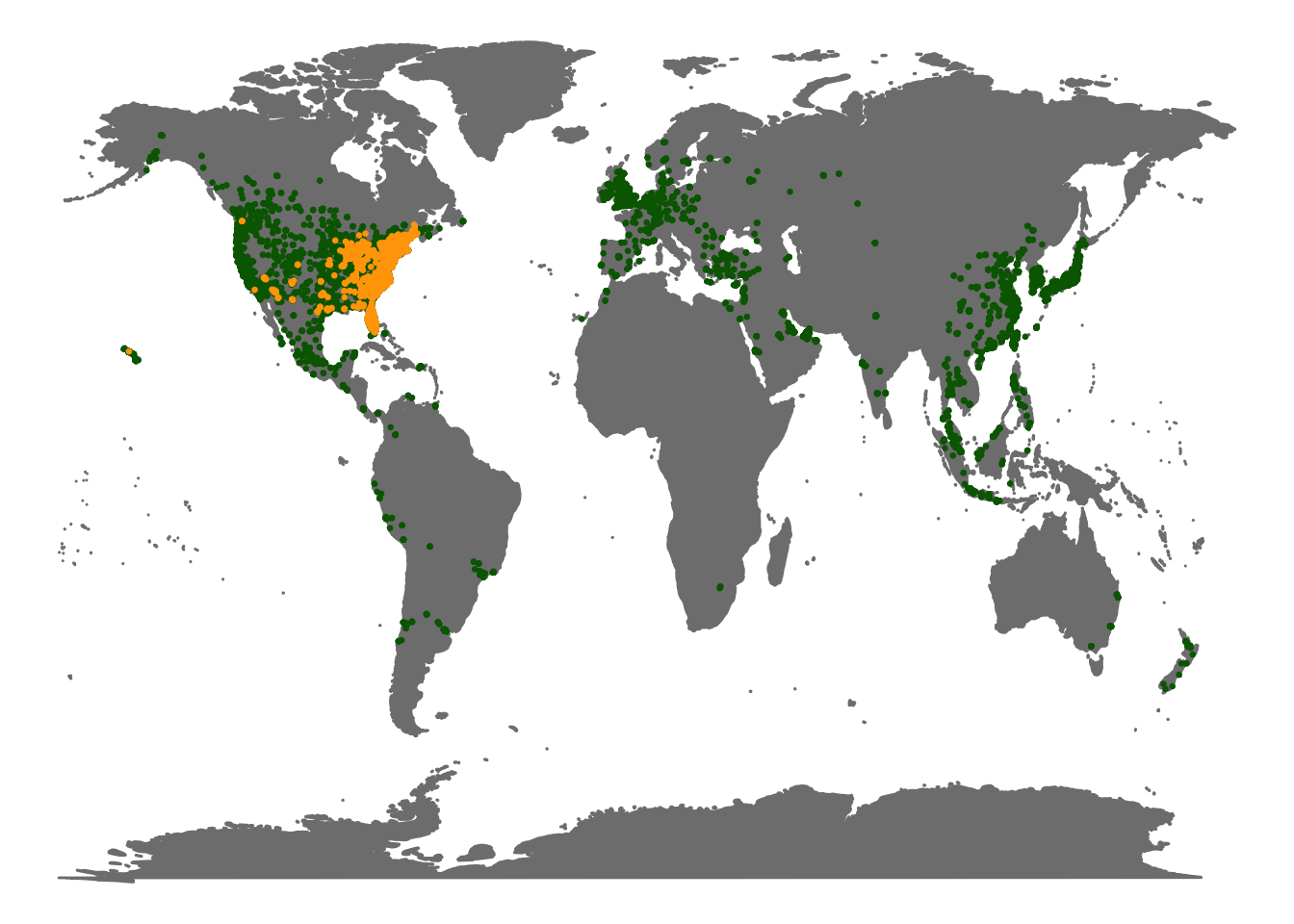
A basic plot of the global Starbucks data.

Code

library(ggmap)
mapWorld <- borders("world", colour="gray50", fill="gray50") # create a layer of borders
mp <- ggplot() +   mapWorld
mp <- mp + geom_point(aes(x=Starbucks$Longitude, y=Starbucks$Latitude) ,color="dark green", size=0.5) + xlab("") + ylab("")
mp <- mp + geom_point(aes(x=Dunkin.Donuts$loc_LONG_centroid, y=Dunkin.Donuts$loc_LAT_centroid) ,color="orange", size=0.5) + xlab("") + ylab("") + theme_void()
mp

Starbucks and Dunkin

Google Maps interface changed and there are limits to what can be geocoded without fees. It can get rather expensive if one is not careful. Let me try this out. The first step is to create the addresses to be geocoded. Let’s look at the Tim.Hortons data.

Code

library(DT)
head(Tim.Hortons) %>% datatable()

I will need to paste/glue them together. I want to paste the address, the city, the state and postal code, then the country but the state and postal code are separate entries so paste them with a space delimiter embedded in the bigger paste command with a comma separation.

Geocoding Tim Horton’s

What follows is the code that I used to create them and to geocode them. I then saved the result and will load it from the saved version.

Code

Tim.Hortons.GC <- Tim.Hortons %>% mutate(full.address=paste(address,city,paste(state, postal_code, sep=" "),toupper(country),sep=", "))
Tim.Hortons.GC <- Tim.Hortons.GC %>% mutate_geocode(full.address, output="latlon")
save(Tim.Hortons.GC, file="data/THGC.RData")

Load the saved and geocoded data

Code

load("data/THGC.RData")
Tim.Hortons.GC <- Tim.Hortons.GC %>% mutate(popup = paste0(store_name,"<br>",address,"<br>",city,", ",state,"<br>",as.character(postal_code),"<br>",toupper(country), sep=""))
head(Tim.Hortons.GC)

Now I want to filter off US locations and create the most basic data structure to map.

Code

THUS <- Tim.Hortons.GC %>% 
  select(country,popup,lon,lat)
names(THUS) <- c("Country","Address","Longitude","Latitude")
THUS$chain <- "Tim Horton's"
head(THUS)

Dunkin Donuts

Thankfully, Dunkin Donuts is already geocoded just as Starbucks was. In this case, I just need some organized data that I can bind together with the same structure as the Tim Horton’s data.

Code

Dunkin.Donuts$PostCode <- as.character(ifelse(length(Dunkin.Donuts$e_postal)==4, paste0("0",Dunkin.Donuts$e_postal),Dunkin.Donuts$e_postal))
Dunkin.Donuts <- Dunkin.Donuts %>% mutate(popup = paste0("Dunkin Donuts <br>",e_address,"<br>",e_city, ", ",e_state,"<br>", PostCode,"<br>",e_country, sep=""))
DDUS <- Dunkin.Donuts %>% select(e_country, popup, loc_LONG_centroid,loc_LAT_centroid)
names(DDUS) <- c("Country","Address","Longitude","Latitude")
DDUS$chain <- "Dunkin"
head(DDUS)

Finally, let me put together a version of the Starbucks data that looks just as the others.

Code

SBUX <- Starbucks %>% select(Country,popup,Longitude,Latitude)
names(SBUX) <- c("Country","Address","Longitude","Latitude")
SBUX$chain <- "Starbucks"
head(SBUX)

With all three of the data sources in a similar format and the like, it is now time to bind them together. There are over 19,000 rows and this would yield 19,000+ popups. That will excessively task resources so, as proof of concept, I will simply sample 300 of them and plot those.

Code

Map.Coffee.Complete <- bind_rows(DDUS,SBUX,THUS) %>% mutate(Country = toupper(Country))
US.Map.Coffee <- Map.Coffee.Complete %>% filter(Country=="US")
US.Map.Coffee <- US.Map.Coffee[c(sample(c(1:19246), size=300, replace=FALSE)),]

Now I have all the data that I need to build the map.
That works as planned.

Code

mp <- leaflet() %>% 
  addTiles() %>%
  addMarkers(~Longitude, ~Latitude, data=US.Map.Coffee, popup=~Address) %>% setView(-94.67, 39.1, zoom = 6)
mp

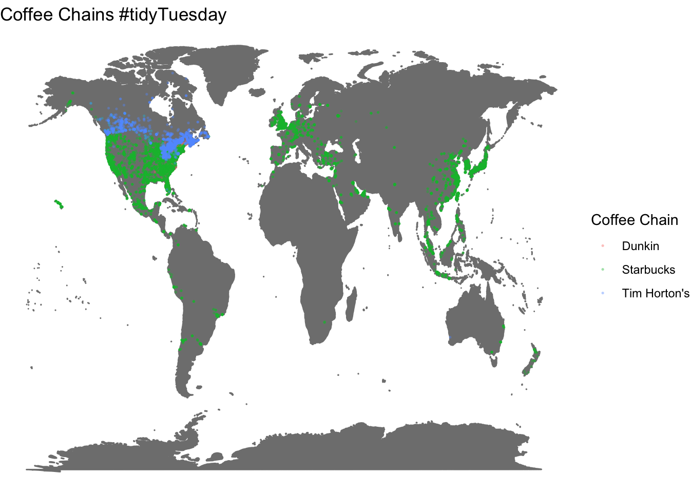
A Full World Map

Code

library(ggmap)
mapWorld <- borders("world", colour="gray50", fill="gray50") # create a layer of borders
mp <- ggplot() + mapWorld
mp <- mp + 
  geom_point(aes(x=Longitude, y=Latitude, color=chain), size=0.3, alpha=0.3, data=Map.Coffee.Complete) + 
  xlab("") + 
  ylab("") + 
  theme_void() + 
  labs(color="Coffee Chain", title="Coffee Chains #tidyTuesday")
mp

References

Code

knitr::write_bib(names(sessionInfo()$otherPkgs), file="bibliography.bib")

References

Cheng, Joe, Bhaskar Karambelkar, and Yihui Xie. 2022. Leaflet: Create Interactive Web Maps with the JavaScript Leaflet Library. https://rstudio.github.io/leaflet/.

Clarke, Erik, Scott Sherrill-Mix, and Charlotte Dawson. 2022. Ggbeeswarm: Categorical Scatter (Violin Point) Plots. https://github.com/eclarke/ggbeeswarm.

Firke, Sam. 2023. Janitor: Simple Tools for Examining and Cleaning Dirty Data. https://CRAN.R-project.org/package=janitor.

Hafen, Ryan. 2020. Geofacet: Ggplot2 Faceting Utilities for Geographical Data. https://github.com/hafen/geofacet.

Kahle, David, and Hadley Wickham. 2013. “Ggmap: Spatial Visualization with Ggplot2.” The R Journal 5 (1): 144–61. https://journal.r-project.org/archive/2013-1/kahle-wickham.pdf.

Kahle, David, Hadley Wickham, and Scott Jackson. 2022. Ggmap: Spatial Visualization with Ggplot2. https://github.com/dkahle/ggmap.

Müller, Kirill, and Hadley Wickham. 2022. Tibble: Simple Data Frames. https://CRAN.R-project.org/package=tibble.

Slowikowski, Kamil. 2023. Ggrepel: Automatically Position Non-Overlapping Text Labels with Ggplot2. https://github.com/slowkow/ggrepel.

Waring, Elin, Michael Quinn, Amelia McNamara, Eduardo Arino de la Rubia, Hao Zhu, and Shannon Ellis. 2022. Skimr: Compact and Flexible Summaries of Data. https://CRAN.R-project.org/package=skimr.

Wickham, Hadley. 2016. Ggplot2: Elegant Graphics for Data Analysis. Springer-Verlag New York. https://ggplot2.tidyverse.org.

———. 2022a. Stringr: Simple, Consistent Wrappers for Common String Operations. https://CRAN.R-project.org/package=stringr.

———. 2022b. Tidyverse: Easily Install and Load the Tidyverse. https://CRAN.R-project.org/package=tidyverse.

———. 2023. Forcats: Tools for Working with Categorical Variables (Factors). https://CRAN.R-project.org/package=forcats.

Wickham, Hadley, Mara Averick, Jennifer Bryan, Winston Chang, Lucy D’Agostino McGowan, Romain François, Garrett Grolemund, et al. 2019. “Welcome to the tidyverse.” Journal of Open Source Software 4 (43): 1686. https://doi.org/10.21105/joss.01686.

Wickham, Hadley, and Jennifer Bryan. 2022. Readxl: Read Excel Files. https://CRAN.R-project.org/package=readxl.

Wickham, Hadley, Winston Chang, Lionel Henry, Thomas Lin Pedersen, Kohske Takahashi, Claus Wilke, Kara Woo, Hiroaki Yutani, and Dewey Dunnington. 2022. Ggplot2: Create Elegant Data Visualisations Using the Grammar of Graphics. https://CRAN.R-project.org/package=ggplot2.

Wickham, Hadley, Romain François, Lionel Henry, Kirill Müller, and Davis Vaughan. 2023. Dplyr: A Grammar of Data Manipulation. https://CRAN.R-project.org/package=dplyr.

Wickham, Hadley, and Lionel Henry. 2023. Purrr: Functional Programming Tools. https://CRAN.R-project.org/package=purrr.

Wickham, Hadley, Jim Hester, and Jennifer Bryan. 2022. Readr: Read Rectangular Text Data. https://CRAN.R-project.org/package=readr.

Wickham, Hadley, Davis Vaughan, and Maximilian Girlich. 2023. Tidyr: Tidy Messy Data. https://CRAN.R-project.org/package=tidyr.

Xie, Yihui, Joe Cheng, and Xianying Tan. 2023. DT: A Wrapper of the JavaScript Library DataTables. https://github.com/rstudio/DT.