Introducing Esquisse

Executing

esquisse:::esquisser(viewer="browser")

NB: It needs to run in a separate browser window.

Selecting Data

What is available in the environment?

A Run Through

Basic Data Visualization

Particularly for qualitative variables, radiant is quite limited.

• One Qualitative Variable
  
• One Quantitative Variable
• Two Qualitative Variables
  
• Two Quantitative Variables
• Visualizing a Mix

One Qualitative Variable

Just filling has no x or y so a bar is the choice.

One Quantity

Options

BoxPlot

Density

Two Qualitative Variables

Fill

Stack

Dodge

Two Quantities are Scatterplots

Mixed Opens Up A Lot

A Violin

A note on scaling….

An Export

Two Geometries

Probability

Why Jaynes?

His approach is intuitive. If you are familiar with probability already, some of you have formal training, Appendix A sets out the key differences.

Why did I ask you to read this? He builds a basic foundation. He derives rules. Those rules are the same rules that we will deploy. But he does it from more basic foundations. Yes, he can do math. That’s not the point; there is a simple representation of all of these ideas. And only a small number of rules that we will define precisely.

Where does Probability Come From?

There are three common sources of probabilities:

• Known formula [Dice, Coins, etc.]
• Empirical frequency
• Subjective belief

Jaynes is a proponent of the latter.

A priori probability

The probability of a given integer on a k-sided die: \frac{1}{k}.

The probability of heads with a fair coin: \frac{1}{2}.

The probability of a Queen? \frac{4}{52}

The probability of a Diamond? \frac{13}{52}

The Queen of Diamonds? \frac{1}{52} or (\frac{4}{52}\times\frac{13}{52})

Quasirandom numbers

Empirical probability: frequency

How often does something happen?

Annie

Straight to Watch

This is Historical Statistics

How likely am I to be admitted? Consult the admissions rate

How fast do I drive? Likelihood of law enforcement and need for speed

In data: this is tables.

Berkeley

        
           No  Yes
  Female 1278  557
  Male   1493 1198

    M.F   No  Yes
 Female 1278  557
   Male 1493 1198

library(tidyverse)
library(janitor)
table(UCBAdmit$M.F,UCBAdmit$Admit)
UCBAdmit %>% tabyl(M.F, Admit)

Three Versions

prop.table(table(UCBAdmit$M.F,UCBAdmit$Admit), 1)

        
                No       Yes
  Female 0.6964578 0.3035422
  Male   0.5548123 0.4451877

prop.table(table(UCBAdmit$M.F,UCBAdmit$Admit), 2)

        
                No       Yes
  Female 0.4612053 0.3173789
  Male   0.5387947 0.6826211

prop.table(table(UCBAdmit$M.F,UCBAdmit$Admit))

        
                No       Yes
  Female 0.2823685 0.1230667
  Male   0.3298719 0.2646929

UCBAdmit %>% tabyl(M.F, Admit) %>% adorn_percentages("row")

    M.F        No       Yes
 Female 0.6964578 0.3035422
   Male 0.5548123 0.4451877

UCBAdmit %>% tabyl(M.F, Admit) %>% adorn_percentages("col")

    M.F        No       Yes
 Female 0.4612053 0.3173789
   Male 0.5387947 0.6826211

UCBAdmit %>% tabyl(M.F, Admit) %>% adorn_percentages("all")

    M.F        No       Yes
 Female 0.2823685 0.1230667
   Male 0.3298719 0.2646929

Plot It

( UCBM <- ggplot(UCBAdmit) + aes(x=M.F, fill=Admit) + geom_bar(position="dodge") + scale_fill_viridis_d() )

More on this later.

Subjective Probability

How likely do we believe something is?

The Great Divide

Empirical frequency vs. subjective belief

Physics Disagrees: We Goin Nova…..

Annie’s a liar.

What matters in group decision making is probably as much the beliefs [subjective] as the evidence [frequency].

How should we reflect this in strategies of argumentation/persuasion?

Think

What matters?

# RUN ME
# may need to install.packages("countdown")
library(countdown)
countdown_fullscreen(
  minutes = 5, seconds = 0,
  margin = "5%",
  font_size = "8em",
)

Three Concepts from Set Theory

• Intersection [and]
• Union [or] avoid double counting the intersection
• Complement [not]

Three Distinct Probabilities

• Joint: Pr(x=x and y=y)
• Marginal: Pr(x=x) or Pr(y=y)
• Conditional: Pr(x=x | y=y) or Pr(y =y | x = x)

Joint Probability

The table sums to one.

For Berkeley:

UCBAdmit %>% tabyl(M.F, Admit) %>% adorn_percentages("all")

    M.F        No       Yes
 Female 0.2823685 0.1230667
   Male 0.3298719 0.2646929

prop.table(table(UCBAdmit$M.F,UCBAdmit$Admit))

        
                No       Yes
  Female 0.2823685 0.1230667
  Male   0.3298719 0.2646929

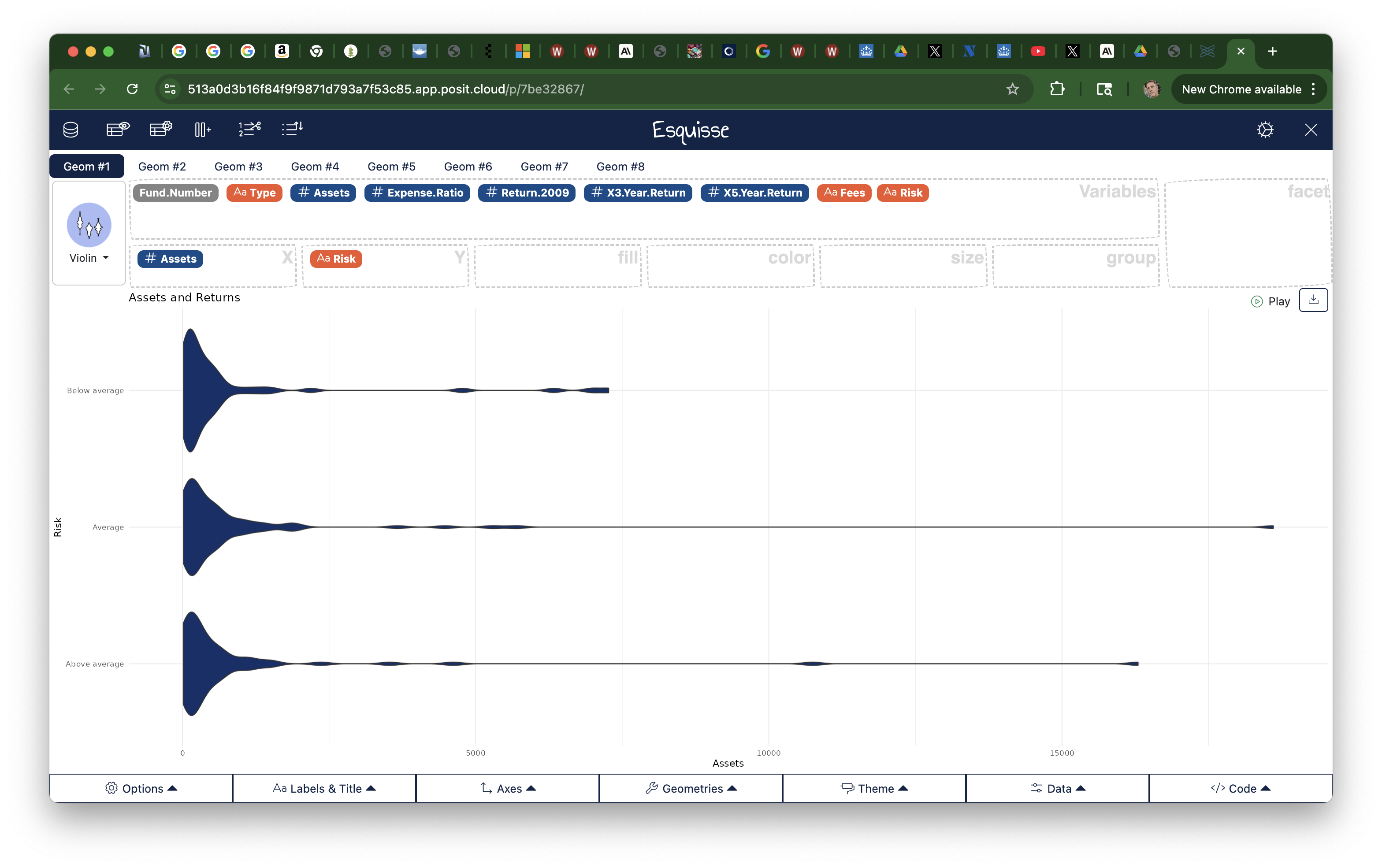
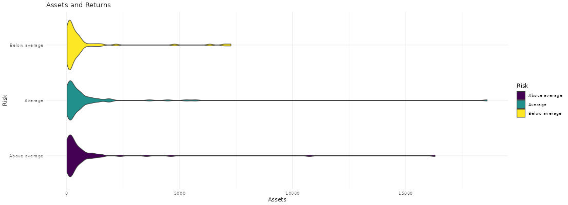
Marginal Probability

The row/column sums to one. We collapse the table to a single margin. Here, two can be identified. The probability of Admit and the probability of M.F.

UCBAdmit %>% tabyl(M.F)

    M.F    n   percent
 Female 1835 0.4054353
   Male 2691 0.5945647

UCBAdmit %>% tabyl(Admit)

 Admit    n   percent
    No 2771 0.6122404
   Yes 1755 0.3877596

prop.table(table(UCBAdmit$M.F))

   Female      Male 
0.4054353 0.5945647 

prop.table(table(UCBAdmit$Admit))

       No       Yes 
0.6122404 0.3877596 

Conditional Probability

How does one margin of the table break down given values of another? Each row or column sums to one

Four can be identified, the probability of admission/rejection for Male, for Female; the probability of male or female for admits/rejects.

For Berkeley:

UCBAdmit %>% tabyl(M.F, Admit) %>% adorn_percentages("row")

    M.F        No       Yes
 Female 0.6964578 0.3035422
   Male 0.5548123 0.4451877

prop.table(table(UCBAdmit$M.F,UCBAdmit$Admit), 1)

        
                No       Yes
  Female 0.6964578 0.3035422
  Male   0.5548123 0.4451877

UCBAdmit %>% tabyl(M.F, Admit) %>% adorn_percentages("col")

    M.F        No       Yes
 Female 0.4612053 0.3173789
   Male 0.5387947 0.6826211

prop.table(table(UCBAdmit$M.F,UCBAdmit$Admit), 2)

        
                No       Yes
  Female 0.4612053 0.3173789
  Male   0.5387947 0.6826211

Law of Total Probability

Is a combination of the distributive property of multiplication and the fact that probabilities sum to one.

For example, the probability of Admitted and Male is the probability of admission for males times the probability of male.

Pr(x=x, y=y) = Pr(y | x)Pr(x)

Or it is the probability of being admitted times the probabilty of being male among admits.

Pr(x=x, y=y) = Pr(x | y)Pr(y)

Now the Substance

ggplot(UCBAdmit) + aes(x=M.F, fill=Admit) + geom_bar() + scale_fill_viridis_d()

Is that an Adequate Comparison?

ggplot(UCBAdmit) + 
  aes(x=M.F, fill=Admit) + 
  geom_bar(position="fill") + 
  scale_fill_viridis_d() + 
  facet_wrap(vars(Dept))

The Magic of Bayes Rule

To find the joint probability [the intersection] of x and y, we can use either of the aforementioned methods. To turn this into a conditional probability, we simply take it is a proportion of the relevant margin.

Pr(x | y) = \frac{Pr(y | x) Pr(x)}{Pr(y)}

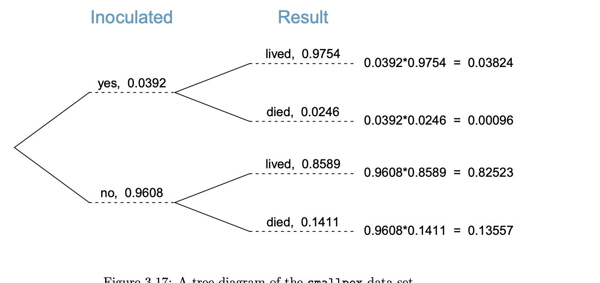
A Bit on Juries

• Start from Section 3.2.7
• The juror’s decision tree

Three nodes: guilty and not at each, convict at the third.

Bayesian Reasoning is Core to Toulmin’s Thinking

Pr(Decision | data) = \frac{Pr(data | Decision) Pr(Decision)}{Pr(Data)}