Grapher

There is commented code for loading in each of the three data files. I have combined them and mutated them because it is a long operation.

library(magrittr)
load("Complete.Data.01.2026.RData")

A few objectives.

• It occurred to me that we do not really make use of the discrete tag. I will in this document in a moment.

Fresh.Outcome

I have recreated the outcomes below in a variable called Fresh.Outcome. We should be careful about how these are recoded to be both transparent about what it does and for our clarity in reporting. Here is that table.

Complete.Data.01.2026$Fresh.Outcome <- c(1:196000) %>% map_chr(., function(x) {Complete.Data.01.2026$response$body$choices[[x]]$message$content})
Complete.Data.01.2026$model <- Complete.Data.01.2026$body$model
Complete.Data.01.2026 <- Complete.Data.01.2026 |> mutate(modelF = factor(model, levels = c('gpt-4-turbo-2024-04-09', 'gpt-4-0613', 'gpt-4o-2024-08-06', 'gpt-5.2-2025-12-11')))
Complete.Data.01.2026 |> group_by(Fresh.Outcome, model) |> summarise(Count = n()) |>  ungroup() |> pivot_wider(names_from = model, values_from = Count) |> gt()

Fresh.Outcome	gpt-5.2-2025-12-11	gpt-4-0613	gpt-4-turbo-2024-04-09	gpt-4o-2024-08-06
	15	NA	NA	NA
Arcsine	36	NA	NA	NA
Bernoulli	744	1071	690	835
Beta	4165	14	8885	2141
Betabinomial	33	NA	NA	NA
Bimodal	NA	49	NA	NA
Binomial	15525	84	1969	1028
Categorical	86	NA	NA	NA
Cauchy	35	NA	6	NA
Chisquare	9	NA	NA	NA
Degenerate	71	71	71	71
ExGaussian	3	NA	NA	NA
Exponential	196	156	930	5266
Gamma	2714	NA	517	17
Geometric	583	NA	NA	NA
Gumbel	76	NA	NA	NA
Laplace	3	NA	454	NA
Log-Normal	NA	NA	NA	3
Log-normal	NA	NA	NA	938
Logistic	NA	NA	7	NA
Lognormal	8127	3979	7974	468
Mixture	1	NA	1	NA
Multinomial	24	NA	NA	NA
NegBinomial	5	NA	NA	NA
Negative Binomial	NA	5	NA	NA
NegativeBinomial	224	4	NA	NA
Negativebinomial	197	NA	NA	NA
Negbinomial	1	NA	NA	NA
Normal	5201	29210	3230	12090
Pareto	83	NA	126	142
Pascal	77	NA	NA	NA
Poisson	8553	12981	22764	17042
Skew-normal	NA	NA	10	NA
Skew-right	NA	3	NA	NA
SkewNormal	NA	NA	160	NA
Skewed	NA	NA	NA	1
Skewness	NA	245	5	NA
Skewnormal	15	NA	3	NA
Student	29	NA	NA	NA
Studentt	1	NA	NA	NA
Triangular	16	NA	1	NA
Uniform	1250	1128	1141	8557
Weibull	78	NA	56	400
ZIP	1	NA	NA	NA
Zero-inflated	NA	NA	NA	1
ZeroInflatedPoisson	4	NA	NA	NA
ZeroinflatedPoisson	8	NA	NA	NA
Zipf	2	NA	NA	NA
arcsine	1	NA	NA	NA
beta	4	NA	NA	NA
binomial	1	NA	NA	NA
categorical	3	NA	NA	NA
exgaussian	1	NA	NA	NA
exponential	3	NA	NA	NA
gamma	33	NA	NA	NA
geometric	3	NA	NA	NA
lognormal	723	NA	NA	NA
negativebinomial	8	NA	NA	NA
normal	11	NA	NA	NA
skewnormal	3	NA	NA	NA
t	13	NA	NA	NA
uniform	2	NA	NA	NA

I am going to recreate the Outcome variable as follows.

Complete.Data.01.2026 <- Complete.Data.01.2026 |> 
  mutate(Outcome = case_match(Fresh.Outcome, 
                              c("arcsine","Arcsine") ~ "Arcsine",
                              c("categorical","Categorical") ~ "Categorical",
                              c("exponential","Exponential") ~ "Exponential",
                              c("beta","Beta") ~ "Beta",
                              c("Chisquare","Chi-Square") ~ "Chi-square",
                              c("exgaussian","ExGaussian") ~ "ExGaussian",
                              c("Normal","normal") ~ "Normal",
                              c("binomial","Binomial") ~ "Binomial",
                              c("geometric","Geometric") ~ "Geometric",
                              c("gamma","Gamma") ~ "Gamma",                              c("Lognormal","lognormal","Log-Normal","Log-normal") ~ "Lognormal",
                              c("NegativeBinomial","Negative Binomial","NegBinomial","Negbinomial","negativebinomial","Negativebinomial") ~ "Negative Binomial",
                              c("Skewed","Skewnormal","SkewNormal","Skew-normal","Skew-right","Skewness","skewnormal")~ "Skewed",
                              c("Student","Studentt","Studentt","t")~ "Student's t", c("Uniform","uniform")~ "Uniform",
                              c("ZeroInflatedPoisson","ZeroinflatedPoisson","Zero-inflated","ZIP")~ "ZIP",
                              .default = Fresh.Outcome))
# Complete.Data |> group_by(Outcome, model) |> summarise(Count = n()) |>  ungroup() |> pivot_wider(names_from = model, values_from = Count) |> gt()

The discrete tag

Complete.Data.01.2026 <- Complete.Data.01.2026 |> mutate(Type = case_match(name, c("Binomial","Geometric","Poisson") ~ "Discrete", .default = "not Discrete"))
Complete.Data.01.2026 <- Complete.Data.01.2026 |> mutate(Correct = as.character(name==Outcome)) |> mutate(Correct = case_match(Correct, "TRUE" ~ "Correct", .default = "Incorrect"))

Basic Percent Correctly Predicted

MNTotals <- Complete.Data.01.2026 |> group_by(model, name) |> summarise(Total = n()) |> ungroup()
PCP <- Complete.Data.01.2026 |> group_by(model, name, Correct) |> summarise(count = n()) |> ungroup()
PCPTab <- left_join(PCP, MNTotals) |> filter(Correct=="Correct") |> mutate(PCP = count / Total) |> select(model, name, PCP)
PCPTab

# A tibble: 29 × 3
   model                  name          PCP
   <chr>                  <chr>       <dbl>
 1 gpt-4-0613             Beta      0.0028 
 2 gpt-4-0613             Binomial  0.00394
 3 gpt-4-0613             Lognormal 0.880  
 4 gpt-4-0613             Normal    1      
 5 gpt-4-0613             Poisson   0.554  
 6 gpt-4-0613             Uniform   0.0002 
 7 gpt-4-turbo-2024-04-09 Beta      0.972  
 8 gpt-4-turbo-2024-04-09 Binomial  0.104  
 9 gpt-4-turbo-2024-04-09 Gamma     0.044  
10 gpt-4-turbo-2024-04-09 Lognormal 0.857  
# ℹ 19 more rows

The Plot

Tab.All <- Complete.Data.01.2026 |> group_by(model, name, Outcome) |> summarise(Count = n()) |> ungroup() |> group_by(model,name) |> mutate(Total = sum(Count)) |> ungroup() |> mutate(PCP = round(Count / Total, digits=3)) |> ungroup()
TAP1 <- Tab.All |> ggplot() + aes(x=Outcome, y=fct_rev(name), fill=PCP, facet=model) + 
    geom_tile(alpha=0.4) + 
    scale_fill_viridis_c(option = "E", alpha=0.4, direction = -1) + 
    labs(y="True Distribution", x="Model Outcome") + geom_text(aes(label=round(PCP, digits=2)), size=3, color="black") + labs(caption="Values are row percents", title="True Distributions and Model Responses", fill="Row. Pct.") + theme_minimal() + theme(legend.location = "plot", panel.spacing = unit(2, "lines"), plot.label= element_text(size=5), plot.title=element_text(size=10, face = "bold", hjust=0), plot.title.position = "plot", axis.text.x = element_text(size=8)) + 
    theme(legend.position="bottom", legend.direction = "horizontal") + facet_wrap(vars(model), nrow = 3, strip.position = "bottom") + scale_x_discrete(position="top", guide = guide_axis(n.dodge = 2)) +
    theme(
        legend.text = element_text(size = 6), 
        legend.title = element_text(size = 8),
        legend.key.width = unit(0.15, "in"),
        legend.position = c(0.15, 0.69)
    )
TAP1

TAP1BL <- Tab.All |> ggplot() + aes(x=Outcome, y=fct_rev(name), fill=PCP, facet=model) + 
    geom_tile(alpha=0.4) + 
    scale_fill_viridis_c(option = "E", alpha=0.4, direction = -1) + 
    labs(y="True Distribution", x="Model Outcome") + geom_text(aes(label=round(PCP, digits=2)), size=3, color="black") + labs(caption="Values are row percents", title="True Distributions and Model Responses", fill="Row. Pct.") + theme_minimal() + theme(legend.location = "plot", panel.spacing = unit(2, "lines"), plot.label= element_text(size=5), plot.title=element_text(size=10, face = "bold", hjust=0), plot.title.position = "plot", axis.text.x = element_text(size=8)) + 
    theme(legend.position="bottom", legend.direction = "horizontal") + facet_wrap(vars(model), nrow = 3, strip.position = "bottom") + scale_x_discrete(position="top", guide = guide_axis(n.dodge = 2)) +
    theme(
        legend.text = element_text(size = 6), 
        legend.title = element_text(size = 8),
        legend.key.width = unit(0.15, "in"),
        legend.position = c(0, -0.06)
    )
TAP1BL

ggsave(filename = "Final-Table-BotLLeg.jpeg", TAP1BL)

TAP1TR <- Tab.All |> ggplot() + aes(x=Outcome, y=fct_rev(name), fill=PCP, facet=model) + 
    geom_tile(alpha=0.4) + 
    scale_fill_viridis_c(option = "E", alpha=0.4, direction = -1) + 
    labs(y="True Distribution", x="Model Outcome") + geom_text(aes(label=round(PCP, digits=2)), size=3, color="black") + labs(caption="Values are row percents", title="True Distributions and Model Responses", fill="Row. Pct.") + theme_minimal() + theme(legend.location = "plot", panel.spacing = unit(2, "lines"), plot.label= element_text(size=5), plot.title=element_text(size=10, face = "bold", hjust=0), plot.title.position = "plot", axis.text.x = element_text(size=8)) + 
    theme(legend.position="bottom", legend.direction = "horizontal") + facet_wrap(vars(model), nrow = 3, strip.position = "bottom") + scale_x_discrete(position="top", guide = guide_axis(n.dodge = 2)) +
    theme(
        legend.text = element_text(size = 6), 
        legend.title = element_text(size = 8),
        legend.key.width = unit(0.15, "in"),
        legend.position = c(0.9, 1.12)
    )
TAP1TR

TAP2 <- Tab.All |> ggplot() + aes(x=Outcome, y=fct_rev(name), fill=PCP, facet=model) + 
    geom_tile(alpha=0.4) + 
    scale_fill_viridis_c(option = "E", alpha=0.4, direction = -1) + 
    labs(y="True Distribution", x="Model Outcome") + geom_text(aes(label=round(PCP, digits=2)), size=3, color="black") + labs(caption="Values are row percents", title="True Distributions and Model Responses", fill="Row. Pct.") + theme_minimal() + theme(legend.location = "plot", panel.spacing = unit(2, "lines"), plot.label= element_text(size=5), plot.title=element_text(size=10, face = "bold", hjust=0), plot.title.position = "plot", axis.text.x = element_text(size=8)) + 
    theme(legend.position="bottom") + facet_wrap(vars(model), nrow = 3, strip.position = "bottom") + scale_x_discrete(position="top", guide = guide_axis(n.dodge = 2)) + 
  theme(
    legend.text = element_text(size = 6), 
    legend.title = element_text(size = 8),
    legend.key.width = unit(0.15, "in"),
    legend.position = c(0.4, 0.8)
    )
TAP2

A go at Discrete

Data.Disc.Tab <- Complete.Data.01.2026 |> filter(Type=="Discrete") |> group_by(model, name, Outcome) |> summarise(Count = n()) |> ungroup() |> group_by(model,name) |> mutate(Total = sum(Count)) |> ungroup() |> mutate(PCP = round(Count / Total, digits=3)) |> ungroup()
TableDisc <- Data.Disc.Tab |> ggplot() + aes(x=Outcome, y=fct_rev(name), fill=PCP, facet=model) + 
    geom_tile(alpha=0.4) + 
    scale_fill_viridis_c(option = "E", alpha=0.4, direction = -1) + 
    labs(y="True Distribution", x="Model Outcome") + geom_text(aes(label=round(PCP, digits=2)), size=3, color="black") + labs(caption="Values are row percents", title="a", subtitle="Discrete Distributions and Model Responses", fill="Row. Pct.") + theme_minimal() + theme(plot.label= element_text(size=5), plot.title=element_text(size=12, face = "bold", hjust=0), plot.title.position = "plot", axis.text.x = element_text(angle = 25)) + 
    theme(legend.position="bottom") + facet_wrap(vars(model), nrow = 3, strip.position = "bottom") + scale_x_discrete(position="top") + guides(fill=FALSE)
TableDisc

TabPCPDisc <- Complete.Data.01.2026 |> filter(Type=="Discrete") |> ggplot() + aes(y=name, fill=as.character(Correct), facet=model) + geom_bar(position="fill", alpha=0.4) + 
    scale_fill_viridis_d(option = "E", alpha=0.4, direction = 1) + 
    labs(y="True Distribution", x="Model Outcome") + labs(title="b", subtitle="True Discrete Distributions and Model Responses", fill="Row. Pct.") + theme_minimal() + theme(plot.title=element_text(size=12, face = "bold", hjust=0), plot.title.position = "plot") + theme(legend.position="bottom") + facet_wrap(vars(model), nrow = 3, strip.position = "bottom") + guides(fill=FALSE)
TabPCPDisc

library(patchwork)
TableDisc + TabPCPDisc + plot_layout(widths=c(5,2))

Not Discrete

Complete.Data.01.2026 |> filter(Type=="not Discrete") |> group_by(model, name, Outcome) |> summarise(Count = n()) |> ungroup() |> group_by(model,name) |> mutate(Total = sum(Count)) |> ungroup() |> mutate(PCP = round(Count / Total, digits=3)) |> ungroup() -> TableDatanD
TableNDisc <- TableDatanD |> ggplot() + aes(x=Outcome, y=fct_rev(name), fill=PCP, facet=model) +
    geom_tile(alpha=0.4) + 
    scale_fill_viridis_c(option = "E", alpha=0.4, direction = -1) + 
    labs(y="True Distribution", x="Model Outcome") + geom_text(aes(label=round(PCP, digits=2)), size=3, color="black") + labs(caption="Values are row percents", title="c", subtitle="Continuous Distributions and Model Responses", fill="Row. Pct.") + theme_minimal() + theme(plot.label= element_text(size=5), plot.title=element_text(size=12, face = "bold", hjust=0), plot.title.position = "plot", axis.text.x = element_text(angle = 25)) + 
    theme(legend.position="bottom") + facet_wrap(vars(model), nrow = 3, strip.position = "bottom") + scale_x_discrete(position="top") + guides(fill=FALSE)
TableNDisc

TabPCPnDisc <- Complete.Data.01.2026 |> filter(Type=="not Discrete") |> ggplot() + aes(y=name, fill=as.character(Correct), facet=model) + geom_bar(position="fill", alpha=0.4) + 
    scale_fill_viridis_d(option = "E", alpha=0.4, direction = 1) + 
    labs(y="True Distribution", x="Model Outcome") + labs(title="d", subtitle="Continuous Distributions and Model Responses", fill="Row. Pct.") + theme_minimal() + theme(plot.title=element_text(size=12, face = "bold", hjust=0), plot.title.position = "plot") + theme(legend.position="bottom") + facet_wrap(vars(model), nrow = 3, strip.position = "bottom") + guides(fill=FALSE)
TabPCPnDisc

A Combined Patchwork

design <- c(area(1,1,4,5),area(1,6,4,8), area(5,1,8,5),area(5,6,8,8))
My.Graph <- (TableDisc + TabPCPDisc) / (TableNDisc + TabPCPnDisc) + plot_layout(guides='collect', design=design, nrow = 2, ncol=2) + theme(legend.position = "bottom")
My.Graph

ggsave(filename = "CoolPlot.png", My.Graph, dpi=600, dev = png, type="cairo", width=9, height=6, units = "in")

gpt4-0613

Tab1.1 <- Complete.Data.01.2026 |> filter(model=="gpt-4-0613") %$% 
  table(name, Outcome) %>% 
  data.frame() %>% group_by(name) %>% 
  mutate(Count = sum(Freq)) %>% ungroup() |> 
  mutate(Percent = round(Freq / Count, digits=3)) |> 
  ggplot() + aes(x=as.character(name), y=as.character(fct_rev(Outcome)), fill=Percent) + 
  geom_tile(alpha=0.4) + 
  scale_fill_viridis_c(option = "E", alpha=0.4, direction = -1) + 
  labs(x="True Distribution", y="gpt-4-0613 Outcome") + geom_text(aes(label=Percent), color="black") + labs(caption="Values are column percents", title="True Distributions and Model Responses", fill="Col. Pct.") + theme_minimal() + theme(plot.title=element_text(size=12, face = "bold", hjust=0), plot.title.position = "plot", axis.text.x = element_text(angle = 45)) + 
  theme(legend.position="bottom")

Tab2.1 <- Complete.Data.01.2026 |> filter(model=="gpt-4-0613") |> group_by(name) |> mutate(Correct = (name==Outcome)) |> ggplot() + aes(x=name, fill=Correct) + geom_bar(position = "fill", alpha=0.4) + scale_fill_viridis_d(option="E", direction=-1) + theme_minimal() + labs(x="True Distribution", y="Percent Correct", title="b", subtitle="Correct Prediction: gpt-4-0613")+ theme(text = element_text(size = 10, family="helvetica"), plot.title = element_text(family="helvetica", face="bold"), plot.title.position = "plot", plot.subtitle = element_text(size=12, family="helvetica"))

Tab3.1 <- Complete.Data.01.2026 |> filter(model=="gpt-4-0613") |> mutate(Correct = (name==Outcome)) |> ggplot() + aes(y=Outcome, fill=Correct) + geom_bar(alpha=0.4, show.legend = FALSE, position = "stack") + scale_fill_viridis_d(option="E", direction=-1) + theme_minimal() + labs(y="gpt-4-0613 Outcome", x="Frequency Chosen", title="c", subtitle="True and False Responses: gpt-4-0613") + theme(text = element_text(size = 10, family="helvetica"), plot.title=element_text(family="helvetica", size=12, face="bold"), plot.title.position = "plot") + theme(legend.position="bottom")

Tab4.1 <- Complete.Data.01.2026 |> filter(model=="gpt-5.2-2025-12-11") |> mutate(Correct = (name==Outcome)) |> ggplot() + aes(y=Outcome, fill=Correct) + geom_bar(alpha=0.4, show.legend = FALSE, position = "stack") + scale_fill_viridis_d(option="E", direction=-1) + theme_minimal() + labs(y="gpt-4-0613 Outcome", x="Frequency Chosen", title="c", subtitle="True and False Responses: gpt-4-0613") + theme(text = element_text(size = 10, family="helvetica"), plot.title=element_text(family="helvetica", size=12, face="bold"), plot.title.position = "plot") + theme(legend.position="bottom")

A third patchwork

design <- c(area(1,1,4,4),area(1,5,4,6), area(5,1,6,4),area(5,5,6,6))
Tab1.1 + Tab3.1 + Tab2.1 + guide_area()+ plot_layout(design=design, guides = "collect") -> Plot3
ggsave("Plot0613A.jpeg", Plot3)

Others

Complete.Data.01.2026 |> ggplot() + aes(y=Outcome, fill=Correct, group=model) + geom_bar(position="fill") + facet_grid(rows=vars(name), cols=vars(model), scales = "free")  + theme_minimal() + scale_fill_viridis_d(option = "E") -> Simples
ggsave("Simples.jpeg", Simples, dpi=600)

Complete.Data.01.2026 |> ggplot() + aes(y=name, fill=Correct) + geom_bar(position="fill", alpha=0.4) + facet_grid(cols=vars(model), scales = "free")  + theme_minimal() + scale_fill_viridis_d(option = "E") + labs(title="a", x="Percent", y="True Distribution", subtitle="Percent Correctly Predicted") + theme(plot.title=element_text(size=12, face = "bold", hjust=0), plot.title.position = "plot", legend.position="bottom") -> Plot1A
Plot1A

Complete.Data.01.2026 |> mutate(NormPoisU = as.character(Outcome %in% c("Uniform","Normal","Poisson"))) |> ggplot() + aes(y=Outcome, fill=Correct) + geom_bar(position="dodge", alpha=0.4) + facet_grid(cols=vars(model), rows=vars(NormPoisU), scales = "free")  + theme_minimal() + scale_fill_viridis_d(option = "E") + labs(title="b", x="Percent", y="Model Outcome", subtitle="Model Outcomes") + theme(plot.title=element_text(size=12, face = "bold", hjust=0), plot.title.position = "plot", legend.position="bottom") -> Plot1B
Plot1B

Complete.Data.01.2026 |> ggplot() + aes(y=Outcome, fill=Correct) + geom_bar(position="dodge", alpha=0.4) + facet_grid(cols=vars(model), scales = "free")  + theme_minimal() + scale_fill_viridis_d(option = "E") + labs(title="b", x="log_10", y="Model Outcome", subtitle="Model Outcomes") + theme(plot.title=element_text(size=12, face = "bold", hjust=0), plot.title.position = "plot", legend.position="bottom") + scale_x_log10() -> Plot1B1
Plot1B1

Complete.Data.01.2026 %$% table(model, name, Outcome, Correct) %>% data.frame() |> ggplot() + aes(y=Outcome, x=Freq, fill=Correct) + geom_col(position="fill") + facet_grid(cols=vars(model))

Complete.Data.01.2026 %$% table(model, name, Outcome, Correct) %>% data.frame() |> ggplot() + aes(y=Outcome, x=Freq, fill=Correct) + geom_col(position="dodge") + facet_grid(cols=vars(model)) + scale_x_sqrt() + scale_fill_viridis_d(option = "E") + theme_minimal()

library(janitor)
DTab <- Complete.Data.01.2026 |> group_by(model, name, Outcome, Correct) |> summarise(Count = n()) |> ungroup() |> group_by(model, name) |> mutate(Total = sum(Count)) |> ungroup() |> mutate(PCP = Count / Total)

TableData |> ggplot() + aes(y=as.character(Outcome), x=as.character(fct_rev(name)), fill=PCP, facet=model) + 
    geom_tile(alpha=0.4) + 
    scale_fill_viridis_c(option = "E", alpha=0.4, direction = -1) + 
    labs(y="True Distribution", x="Model Outcome") + geom_text(aes(label=round(PCP, digits=2)), color="black") + labs(caption="Values are column percents", title="a", subtitle="True Distributions and Model Responses", fill="Col. Pct.") + theme_minimal() + theme(plot.label= element_text(size=5), plot.title=element_text(size=12, face = "bold", hjust=0), plot.title.position = "plot", axis.text.x = element_text(angle = 45)) + 
    theme(legend.position="bottom") + facet_wrap(vars(model), ncol = 3)

addSmallLegend <- function(myPlot, pointSize = 0.5, textSize = 3, spaceLegend = 0.1) {
    myPlot +
        guides(shape = guide_legend(override.aes = list(size = pointSize)),
               color = guide_legend(override.aes = list(size = pointSize))) +
        theme(legend.title = element_text(size = textSize), 
              legend.text  = element_text(size = textSize),
              legend.key.size = unit(spaceLegend, "lines"))
}

# Apply on original plot
addSmallLegend(p)

quartz_off_screen 
                2 

quartz_off_screen 
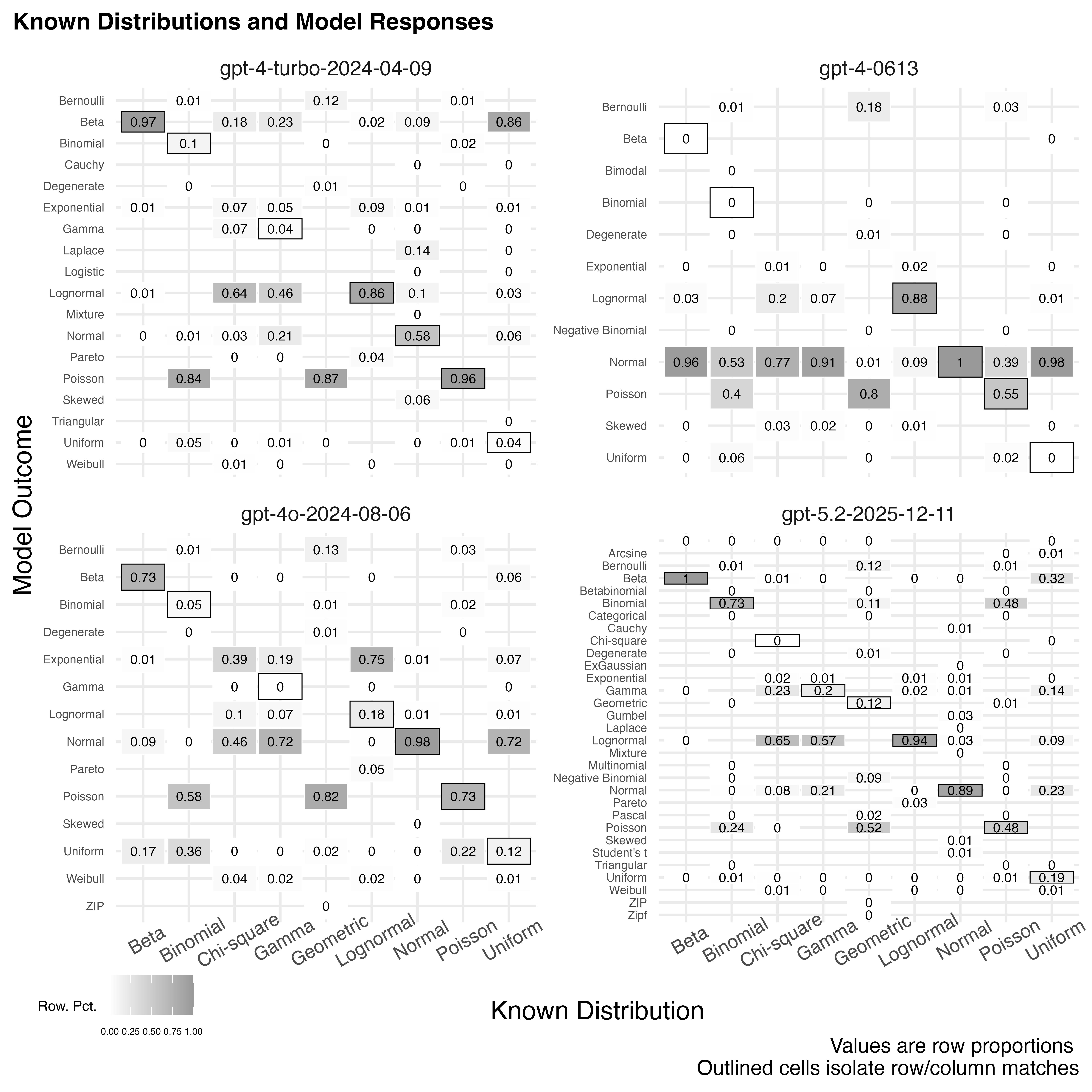
                2 

ggplot(Tab.All) + 
  aes(y=fct_rev(Outcome), x=name, fill=PCP, facet=modelF) + 
  geom_tile(aes(color=Dist.Match), lwd=0.2, width=0.95, height=0.95) + 
  scale_color_manual(values = c("white","black")) + 
  guides(color="none") +
  scale_fill_gradientn(colors = my_greys) + 
  labs(x="Known Distribution", y="Model Outcome") +
  geom_text(aes(label=round(PCP, digits=2)), size=2, color="black") +
  labs(caption="Values are row proportions \n Outlined cells isolate row/column matches", title="Known Distributions and Model Responses", fill="Row. Pct.") + 
  theme_minimal() + 
  theme(legend.location = "plot", 
        panel.spacing = unit(0.5, "lines"), 
        plot.label= element_text(size=5), 
        plot.title=element_text(size=10, face = "bold", hjust=0),
        plot.title.position = "plot", 
        axis.text.x = element_text(size=8, angle=30), 
        axis.text.y = element_text(size=5), 
        legend.direction = "horizontal",
        legend.text = element_text(size = 4), 
        legend.title = element_text(size = 6),
        legend.key.width = unit(0.1, "in"),
        legend.position = c(0.0, -0.1)
) +
    facet_wrap(vars(modelF), scales="free_y")

FinalFig

Round to 3

ggplot(Tab.All) + 
  aes(y=fct_rev(Outcome), x=name, fill=PCP, facet=modelF) + 
  geom_tile(aes(color=Dist.Match), lwd=0.2, width=0.95, height=0.95) + 
  scale_color_manual(values = c("white","black")) + 
  guides(color="none") +
  scale_fill_gradientn(colors = my_greys) + 
  labs(x="Known Distribution", y="Model Outcome") +
  geom_text(aes(label=round(PCP, digits=4)), size=2, color="black") +
  labs(caption="Values are row proportions \n Outlined cells isolate row/column matches", title="Known Distributions and Model Responses", fill="Row. Pct.") + 
  theme_minimal() + 
  theme(legend.location = "plot", 
        panel.spacing = unit(0.5, "lines"), 
        plot.label= element_text(size=5), 
        plot.title=element_text(size=10, face = "bold", hjust=0),
        plot.title.position = "plot", 
        axis.text.x = element_text(size=8, angle=30), 
        axis.text.y = element_text(size=5), 
        legend.direction = "horizontal",
        legend.text = element_text(size = 4), 
        legend.title = element_text(size = 6),
        legend.key.width = unit(0.1, "in"),
        legend.position = c(0.0, -0.1)
) +
    facet_wrap(vars(modelF), scales="free_y")

Tab.All <- Tab.All |> mutate(PCPa = round(PCP, digits=2))
Tab.All$PCPa1 <- as.character(Tab.All$PCPa)
Tab.All <- Tab.All |> mutate(PCPa1 = case_when(PCPa1 == "0" ~ "<0.01", .default = PCPa1))
FF3 <- ggplot(Tab.All) + 
  aes(y=fct_rev(Outcome), x=name, fill=PCP, facet=modelF) + 
  geom_tile(aes(color=Dist.Match), lwd=0.2, width=0.95, height=0.95) + 
  scale_color_manual(values = c("white","black")) + 
  guides(color="none") +
  scale_fill_gradientn(colors = my_greys) + 
  labs(x="Known Distribution", y="Model Outcome") +
  geom_text(aes(label=PCPa1), size=2, color="black") +
  labs(caption="Values are row proportions \n Outlined cells isolate row/column matches", title="Known Distributions and Model Responses", fill="Row. Pct.") + 
  theme_minimal() + 
  theme(legend.location = "plot", 
        panel.spacing = unit(0.5, "lines"), 
        plot.label= element_text(size=5), 
        plot.title=element_text(size=10, face = "bold", hjust=0),
        plot.title.position = "plot", 
        axis.text.x = element_text(size=8, angle=30), 
        axis.text.y = element_text(size=5), 
        legend.direction = "horizontal",
        legend.text = element_text(size = 4), 
        legend.title = element_text(size = 6),
        legend.key.width = unit(0.1, "in"),
        legend.position = c(0.0, -0.1)
) +
    facet_wrap(vars(modelF), scales="free_y")
ggsave(FF3, filename="FinalFigureFreeY-v2.jpeg", width=6.5, height=6.5, dpi=900, units="in")

References

knitr::write_bib(names(sessionInfo()$otherPkgs), file="bibliography.bib")

References

Bache, Stefan Milton, and Hadley Wickham. 2025. Magrittr: A Forward-Pipe Operator for r. https://magrittr.tidyverse.org.

Firke, Sam. 2024. Janitor: Simple Tools for Examining and Cleaning Dirty Data. https://github.com/sfirke/janitor.

Grolemund, Garrett, and Hadley Wickham. 2011. “Dates and Times Made Easy with lubridate.” Journal of Statistical Software 40 (3): 1–25. https://www.jstatsoft.org/v40/i03/.

Iannone, Richard, Joe Cheng, Barret Schloerke, Shannon Haughton, Ellis Hughes, Alexandra Lauer, Romain François, JooYoung Seo, Ken Brevoort, and Olivier Roy. 2025. Gt: Easily Create Presentation-Ready Display Tables. https://gt.rstudio.com.

Mock, Thomas. 2025. gtExtras: Extending Gt for Beautiful HTML Tables. https://github.com/jthomasmock/gtExtras.

Müller, Kirill, and Hadley Wickham. 2026. Tibble: Simple Data Frames. https://tibble.tidyverse.org/.

Pedersen, Thomas Lin. 2025. Patchwork: The Composer of Plots. https://patchwork.data-imaginist.com.

Scheinin, Ilari. 2019. Rasterpdf: Plot Raster Graphics in PDF Files. https://ilarischeinin.github.io/rasterpdf.

Spinu, Vitalie, Garrett Grolemund, and Hadley Wickham. 2024. Lubridate: Make Dealing with Dates a Little Easier. https://lubridate.tidyverse.org.

Urbanek, Simon, and Jeffrey Horner. 2025. Cairo: R Graphics Device Using Cairo Graphics Library for Creating High-Quality Bitmap (PNG, JPEG, TIFF), Vector (PDF, SVG, PostScript) and Display (X11 and Win32) Output. http://www.rforge.net/Cairo/.

Wickham, Hadley. 2016. Ggplot2: Elegant Graphics for Data Analysis. Springer-Verlag New York. https://ggplot2.tidyverse.org.

———. 2023. Tidyverse: Easily Install and Load the Tidyverse. https://tidyverse.tidyverse.org.

———. 2025a. Forcats: Tools for Working with Categorical Variables (Factors). https://forcats.tidyverse.org/.

———. 2025b. Stringr: Simple, Consistent Wrappers for Common String Operations. https://stringr.tidyverse.org.

Wickham, Hadley, Mara Averick, Jennifer Bryan, Winston Chang, Lucy D’Agostino McGowan, Romain François, Garrett Grolemund, et al. 2019. “Welcome to the tidyverse.” Journal of Open Source Software 4 (43): 1686. https://doi.org/10.21105/joss.01686.

Wickham, Hadley, Winston Chang, Lionel Henry, Thomas Lin Pedersen, Kohske Takahashi, Claus Wilke, Kara Woo, Hiroaki Yutani, Dewey Dunnington, and Teun van den Brand. 2025. Ggplot2: Create Elegant Data Visualisations Using the Grammar of Graphics. https://ggplot2.tidyverse.org.

Wickham, Hadley, Romain François, Lionel Henry, Kirill Müller, and Davis Vaughan. 2023. Dplyr: A Grammar of Data Manipulation. https://dplyr.tidyverse.org.

Wickham, Hadley, and Lionel Henry. 2026. Purrr: Functional Programming Tools. https://purrr.tidyverse.org/.

Wickham, Hadley, Lionel Henry, Thomas Lin Pedersen, T Jake Luciani, Matthieu Decorde, and Vaudor Lise. 2025. Svglite: An SVG Graphics Device. https://svglite.r-lib.org.

Wickham, Hadley, Jim Hester, and Jennifer Bryan. 2025. Readr: Read Rectangular Text Data. https://readr.tidyverse.org.

Wickham, Hadley, Davis Vaughan, and Maximilian Girlich. 2025. Tidyr: Tidy Messy Data. https://tidyr.tidyverse.org.