It is probably better posed as, what can we learn from data?
The Big Idea
Inference
In the most basic form, learning something about data that we do not have from data that we do. In the jargon of statistics, we characterize the probability distribution of some feature of the population of interest from a sample drawn randomly from that population.
Quantities of Interest:
Single Proportion: The probability of some qualitative outcome with appropriate uncertainty.1
Single Mean: The average of some quantitative outcome with appropriate uncertainty.1
The Big Idea
Inference
In the most basic form, learning something about data that we do not have from data that we do. In the jargon of statistics, we characterize the probability distribution of some feature of the population of interest from a sample drawn randomly from that population.
Quantities of Interest:
Compare Proportions: Compare key probabilities across two groups with appropriate uncertainty.1
Compare Means: Compare averages/means across two groups with appropriate uncertainty.1
The Big Idea
Inference
In the most basic form, learning something about data that we do not have from data that we do. In the jargon of statistics, we characterize the probability distribution of some feature of the population of interest from a sample drawn randomly from that population.
Study Planning
Plan studies of adequate size to assess key probabilities of interest.
Inference for Data
Of two forms:
Binary/Qualitative
Quantitative
We will first focus first on the former. But before we do, one new concept.
The standard error
It is the degree of variability of a statistic just as the standard deviation is the variability in data.
The standard error of a proportion is \sqrt{\frac{\pi(1-\pi)}{n}} while the standard deviation of a binomial sample would be \sqrt{n*\pi(1-\pi)}.
The standard deviation of a sample is s while the standard error of the mean is \frac{s}{\sqrt{n}}. The average has less variability than the data and it shrinks as n increases.
Let’s think about an election….
Consider election season. The key to modeling the winner of a presidential election is the electoral college in the United States. In almost all cases, this involves a series of binomial variables.
Almost all states award electors for the statewide winner of the election and DC has electoral votes.
We have polls that give us likely vote percentages at the state level. Call it p.win for the probability of winning. We can then deploy rbinom(1000, size=1, p.win) to derive a hypothetical election.
Rinse and repeat to calculate a hypothetical electoral college winner. But how do we calculate p-win?
We infer it from polling data
Qualitative: The Binomial
Is entirely defined by two parameters, n – the number of subjects – and \pi – the probability of a positive response. The probability of exactly x positive responses is given by:
The binomial is the canonical distribution for binary outcomes. Assuming all n subjects are alike and the outcome occurs with \pi probability,1 then we must have a sample from a binomial. A binomial with n=1 is known as a Bernoulli trial
Features of the Binomial
Two key features:
Expectation: n \cdot \pi or number of subjects times probability, \pi \textrm{ if } n=1.
Variance is n \cdot \pi \cdot (1 - \pi) or \pi(1-\pi) \textrm{ if } n=1 and standard deviation is \sqrt{n \cdot \pi \cdot (1 - \pi)} or \sqrt{\pi(1-\pi)} \textrm{ if } n=1.
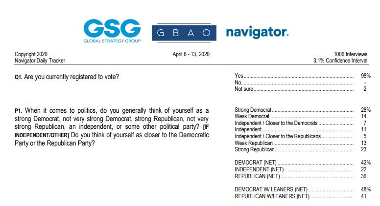
What is the probability of being admitted to UC Berkeley Graduate School?1
I have three variables:
Admitted or not
Gender
The department an applicant applied to.
Admission is the key.
Code
library(janitor) #<<UCBTab <-data.frame(UCBAdmissions) %>% reshape::untable(., .$Freq) %>%select(-Freq)UCBTab %>%tabyl(Admit) # Could also use UCBTab %$% table(Admit)
    Admit    n percent
 Admitted 1755   0.388
 Rejected 2771   0.612
The proportion is denoted as \hat{p}. We can also do this with table.
    Exact binomial test

data:  .
number of successes = 1755, number of trials = 4526, p-value
<2e-16
alternative hypothesis: true probability of success is not equal to 0.5
90 percent confidence interval:
 0.376 0.400
sample estimates:
probability of success
                 0.388
With 90% probability, now often referred to as 90% confidence to avoid using the word probability twice, the probability of being admitted ranges between 0.3758 and 0.3998.
    Exact binomial test

data:  .
number of successes = 1755, number of trials = 4526, p-value
<2e-16
alternative hypothesis: true probability of success is not equal to 0.5
90 percent confidence interval:
 0.376 0.400
sample estimates:
probability of success
                 0.388
Binomial.Search <-data.frame(x =seq(0.33, 0.43, by =0.001)) %>%mutate(Too.Low =pbinom(1755, 1755+2771, x), Too.High =1-pbinom(1754,1755+2771, x))Binomial.Search %>%pivot_longer(cols =c(Too.Low, Too.High)) %>%ggplot(., aes(x = x, y = value, color = name)) +geom_line() +geom_hline(aes(yintercept =0.05)) +geom_hline(aes(yintercept =0.95)) +geom_vline(data = Plot.Me, aes(xintercept = .),linetype =3) +labs(title ="Using the Binomial to Search", color ="Greater/Lesser",x =expression(pi), y ="Probability")
A Third Way: The normal approximation
As long as n and \pi are sufficiently large, we can approximate this with a normal distribution. This will also prove handy for a related reason.
As long as n*\pi > 10, we can write that a standard normal z describes the distribution of \pi, given n – the sample size and \hat{p} – the proportion of yes’s/true’s in the sample.
Pr(\pi) = \hat{p} \pm z \cdot \left( \sqrt{\frac{\hat{p}*(1-\hat{p})}{n}} \right)
R implements this in prop.test. By default, R implements a modified version that corrects for discreteness/continuity. To get the above formula exactly, prop.test(table, correct=FALSE).
A first look at hypotheses
z = \frac{\hat{p} - \pi}{\sqrt{\frac{\pi(1-\pi)}{n}}}
With some proportion calculated from data \hat{p} and some claim about \pi – hereafter called an hypothesis – we can use z to calculate/evaluate the claim. These claims are hypothetical values of \pi. They can be evaluated against a specific alternative considered in three ways:
two-sided, that is \pi = value against not equal.
\pi \geq value against something smaller.
\pi \leq value against something greater.
In the first case, either much bigger or much smaller values could be evidence against equal. The second and third cases are always about smaller and bigger; they are one-sided.
Just as z has metric standard deviations now referred to as standard errors of the proportion, the z here will measure where the data fall with respect to the hypothetical \pi.
With z sufficiently large, and in the proper direction, our hypothetical \pi becomes unlikely given the evidence and should be dismissed.
Three hypothesis tests
Code
(Z.ALL <- (0.3877596-0.5)/(sqrt(0.5^2/4526))) # Calculate z
[1] -15.1
The estimate is 15.1 standard errors below the hypothesized value.
Two Sided
\pi = 0.5 against \pi \neq 0.5.
Code
pnorm(-abs(Z.ALL)) + (1-pnorm(abs(Z.ALL)))
[1] 7.85e-52
Any |z| > 1.64 – probability 0.05 above and below – is sufficient to dispense with the hypothesis.
    1-sample proportions test without continuity correction

data:  table(UCBTab$Admit), null probability 0.5
X-squared = 228, df = 1, p-value <2e-16
alternative hypothesis: true p is not equal to 0.5
90 percent confidence interval:
 0.376 0.400
sample estimates:
    p
0.388
R reports the result as z^2 not z which is \chi^2 not normal; we can obtain the z by taking a square root: \sqrt{228.08} \approx 15.1
This approximation yields an estimate of \pi, with 90% confidence, that ranges between 0.376 and 0.4.
A Cool Consequence of Normal
The formal equation defines:
z = \frac{\hat{p} - \pi}{\sqrt{\frac{\pi(1-\pi)}{n}}}
Some language:
Margin of error is \hat{p} - \pi. [MOE]
Confidence: the probability coverage given z [two-sided].
We need a guess at the true \pi because variance/std. dev. depend on \pi. 0.5 is common because it maximizes the variance; we will have enough no matter what the true value.
Algebra allows us to solve for n.
n = \frac{z^2 \cdot \pi(1-\pi)}{(\hat{p} - \pi)^2}
Example
Estimate the probability of supporting an initiative to within 0.03 with 95% confidence. Assume that the probability is 0.5 [it maximizes the variance and renders a conservative estimate – an upper bound on the sample size]
The probability of admission ranges from 0.376 to 0.4.
If we wish to express this using the normal approximation, a central interval is the observed proportion plus/minus z times the standard error of the proportion – SE(\hat{p}) = \sqrt{\frac{\hat{p}(1-\hat{p})}{n}} NB: The sample value replaces our assumed true value because \pi is to be solved for. For 90%, the probability of admissions ranges from
    Exact binomial test

data:  .
number of successes = 1198, number of trials = 2691, p-value =
0.00000001
alternative hypothesis: true probability of success is not equal to 0.5
90 percent confidence interval:
 0.429 0.461
sample estimates:
probability of success
                 0.445
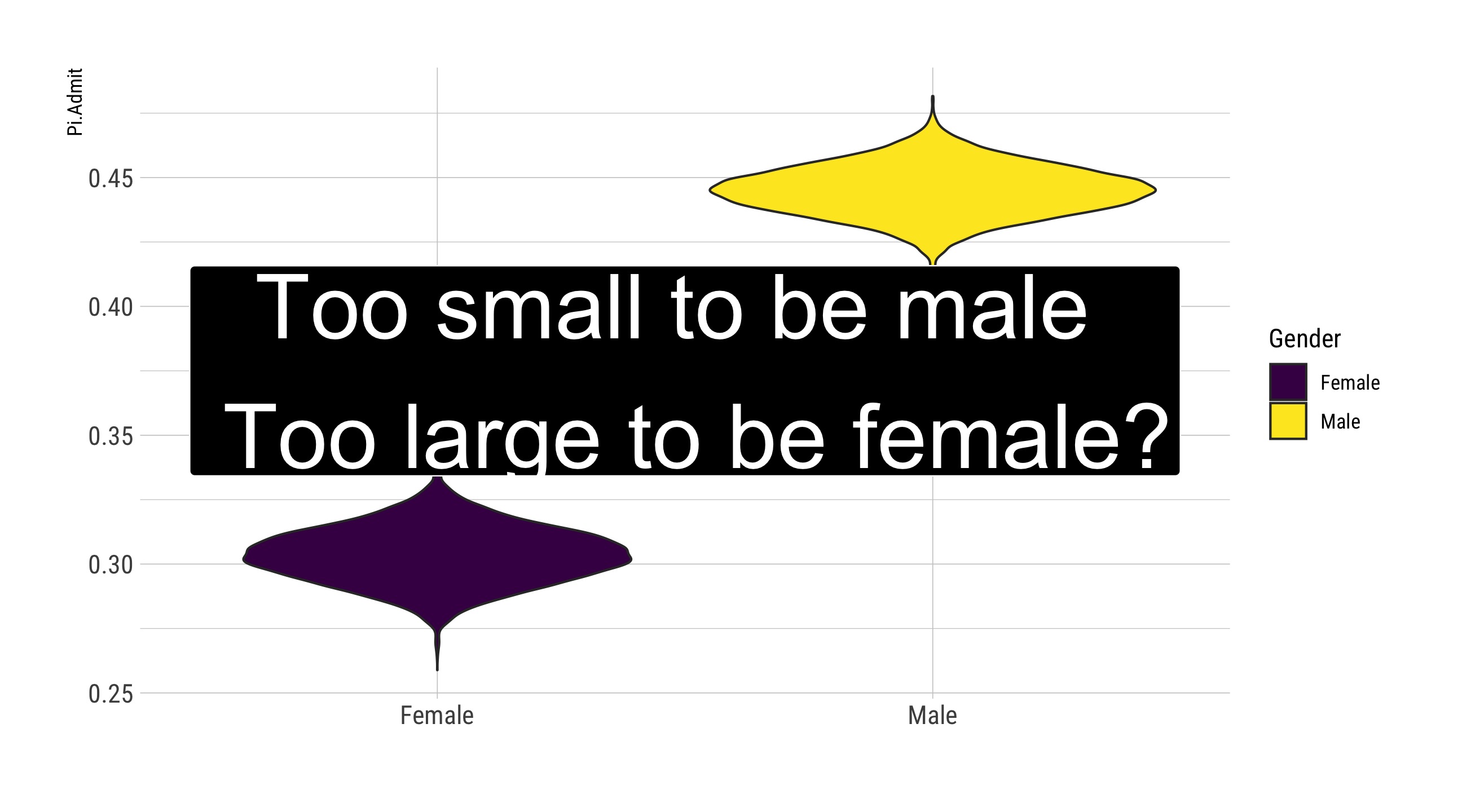
The probability of being admitted, conditional on being Male, ranges from 0.43 to 0.46 with 90% confidence.
    Exact binomial test

data:  .
number of successes = 557, number of trials = 1835, p-value <2e-16
alternative hypothesis: true probability of success is not equal to 0.5
90 percent confidence interval:
 0.286 0.322
sample estimates:
probability of success
                 0.304
The probability of being of Admitted, given a Female, ranges from 0.286 to 0.322 with 90% confidence.
Female: from 0.286 to 0.322
Male: from 0.43 to 0.46
All: from 0.3758 to 0.3998
A Key Visual
Code
UCB.Pi <-bind_rows(UCBTF.Pi, UCBTM.Pi)UCB.Pi %>%ggplot(., aes(x = Gender, y = Pi.Admit, fill = Gender)) +geom_violin() +geom_label(aes(x =1.5, y =0.375), label ="Too small to be male \n Too large to be female?",size =14, fill ="black", color ="white", inherit.aes =FALSE) +guides(size ="none") +labs(x ="") +scale_fill_viridis_d()
    2-sample test for equality of proportions without continuity
    correction

data:  .
X-squared = 92, df = 1, p-value <2e-16
alternative hypothesis: two.sided
90 percent confidence interval:
 0.118 0.165
sample estimates:
prop 1 prop 2
 0.445  0.304
With 90% confidence, a Female is 0.118 to 0.165 [0.1416] less likely to be admitted.
The Standard Error of the Difference
Following something akin to the FOIL method, we can show that the variance of a difference in two random variables is the sum of the variances minus twice the covariance between them.
Var(X - Y) = Var(X) + Var(Y) - 2*Cov(X,Y)
If we assume [or recognize it is generally unknownable] that the male and female samples are independent, the covariance is zero, and the variance of the difference is simply the sum of the variance for male and female, respectively, and zero covariance.
The sum of k squared standard normal (z or Normal(0,1)) variates has a \chi^2 distribution with k degrees of freedom. Two sample tests of proportions can be reported using the chi-square metric as well. R’s prop.test does this by default.
Inference for Data
Of two forms:
Binary/Qualitative (Proportions)
Quantitative (Means)
We will now turn to the latter.
Inference for Quantitative Data
The central limit theorem – or, more aptly, central limit theorems – demonstrates that the sample mean is normally distributed under some – varying – set of conditions.
Let’s Have a Brief Look
Uniform
Code
library(radiant)result <-clt(dist ="Uniform", m =1000)plot(result, stat ="mean", bins =50)
Exponential
Code
result <-clt(dist ="Exponential", m =1000, expo_rate =4)plot(result, stat ="mean", bins =50)
Application: Expenditures
What is the average level of expenditure by Ethnicity?
Why do we focus on the average? Under general conditions, the average has a known probability distribution even if the distribution of the underlying data is unknown. This is a result of the central limit theorem and a generic property of averaging. We can derive this distribution, it is known as t and has one parameter: degrees of freedom.
The t distribution
Results from the combination of a normal random variable in the numerator and a \chi^2 random variable in the denominator. Both should generically hold from the central limit theorem.
Student’s t distribution generically describes the distribution of the difference between a sample mean and the true mean.
BasePlot +geom_area(data = ResQD, aes(x = ResQ, y = Height2), fill ="blue",color ="blue", alpha =0.2, outline.type ="full")
A Parametric Alternative
Under general conditions, the sample and population mean can be described by the t_{df} distribution with a single parameter – degrees of freedom [df] – and metric standard errors of the mean: \frac{s}{\sqrt{n}} as follows:
Given any observed sample of data, only two features of the aforementioned equation remain unknown: \mu – the true mean – and t_{df}. Solving for \mu yields:
    One Sample t-test

data:  Expenditures
t = 26, df = 776, p-value <2e-16
alternative hypothesis: true mean is not equal to 0
90 percent confidence interval:
 16944 19258
sample estimates:
mean of x
    18101
With 90% confidence, average expenditures [for White not Hispanic and Hispanic] range between 1.694^{4} and 1.926^{4} dollars per DDS client.
Disparities in Expenditures?
Code
ggplot(WH, aes(x = Ethnicity, y = Expenditures, fill = Ethnicity)) +geom_violin() +theme_ipsum_rc()
Two Groups?
Code
WH %>%filter(Ethnicity =="White not Hispanic") %$%t.test(Expenditures, conf.level =0.9)
    One Sample t-test

data:  Expenditures
t = 24, df = 400, p-value <2e-16
alternative hypothesis: true mean is not equal to 0
90 percent confidence interval:
 23001 26394
sample estimates:
mean of x
    24698
    One Sample t-test

data:  Expenditures
t = 14, df = 375, p-value <2e-16
alternative hypothesis: true mean is not equal to 0
90 percent confidence interval:
  9736 12395
sample estimates:
mean of x
    11066
Comparing Means
There are two [generic] ways to compare means:
1. The resampling approach
2. t-tests
Comparing Means by Resampling
The method is similar to the approach for comparing proportions. We will:
1. Take a random sample of the same size as the original for each group with replacement.
2. Calculate the average for each group and the difference in the averages.
3. Repeat steps 1 and 2 k times for k samples.
The Resampling Distribution of the Difference
Code
WNHExp <- Discrimination %>%filter(Ethnicity %in%c("White not Hispanic"))HExp <- Discrimination %>%filter(Ethnicity %in%c("Hispanic"))Expenditure.Difference <-data.frame(Diff = ResampleProps::ResampleDiffMeans(WNHExp$Expenditures, HExp$Expenditures))Expenditure.Difference %>%ggplot(., aes(x = Diff)) +geom_density() +theme_minimal() +labs(x ="Average Difference in Average White and Hispanic Expenditures")
The t-test
For independent samples, the Behrens-Fisher problem dictates that comparisons of means have implications for the variance that must be reconciled. In short, we must assume that the variance and standard deviation of the samples are either the same [t] or different [Welch – the default].
In Welch’s case, the standard error is given by:
s_{\overline{x_{1}} - \overline{x_{2}}} = \sqrt{\frac{s^{2}_{1}}{n_{1}} + \frac{s^{2}_{2}}{n_{2}}} though the degrees of freedom follow a formula that involves the kurtosis of the samples [s^{4}].
Code
Discrimination %>%filter(Ethnicity %in%c("White not Hispanic", "Hispanic")) %>%t.test(Expenditures ~ Ethnicity, data = ., conf.lev =0.9)
    Welch Two Sample t-test

data:  Expenditures by Ethnicity
t = -10, df = 743, p-value <2e-16
alternative hypothesis: true difference in means between group Hispanic and group White not Hispanic is not equal to 0
90 percent confidence interval:
 -15785 -11479
sample estimates:
          mean in group Hispanic mean in group White not Hispanic
                           11066                            24698
Code
Discrimination %>%filter(Ethnicity %in%c("White not Hispanic", "Hispanic")) %>%t.test(Expenditures ~ Ethnicity, data = ., conf.lev =0.9, var.equal =TRUE)
    Two Sample t-test

data:  Expenditures by Ethnicity
t = -10, df = 775, p-value <2e-16
alternative hypothesis: true difference in means between group Hispanic and group White not Hispanic is not equal to 0
90 percent confidence interval:
 -15803 -11461
sample estimates:
          mean in group Hispanic mean in group White not Hispanic
                           11066                            24698
Paired t-test
Twinsberg
The paired t-test is a single sample average applied to the measured difference. The key is knowing who is matched with whom and believing that there is at least some variation in both outcomes that depends on the unit in question.
There is a linguistic distinction; this is an average difference instead of the previous difference in averages. The language describes the order of operation. For the paired comparison, I must know what to subtract from what.
Take the example of Concrete.
Twelve distinct batches of concrete are subjected to an additive. Does the additive strengthen concrete?
Code
Concrete %>%datatable()
The Average Difference
For each batch, we can calculate the difference between those with and without an additive. To do so, we need mutate. Let’s plot it.
    One Sample t-test

data:  Concrete$Difference
t = 3, df = 11, p-value = 0.01
alternative hypothesis: true mean is not equal to 0
95 percent confidence interval:
  37.3 279.4
sample estimates:
mean of x
      158
With 95% confidence, the additive increases the average break-weight of the concrete by 37.3 to 279.4 pounds.
An Inference Map
With proportions: If we claim a value of \pi, then use it for the standard error. If not, use the data.
With quantities: If comparing them, are samples independent or dependent? All the relevant quantities are known [or assumed] functions of the data.
For differences, the magic number is nearly always zero – no difference.
Independent: t.test(x, y, alternative="?", mu=0, conf.level=0.95, paired=FALSE, var.equal=FALSE)
Paired: t.test(x, y, alternative="?", mu=0, conf.level=0.95, paired=TRUE)
```
A Workflow
Do we want an hypothesis test or a confidence interval?
Choose a level of confidence/significance/probability.
If hypothesis test, derive the relevant critical value by combining the reference distribution with the level of confidence/significance/probability. What value of z or t would be required to reject the hypothesis? If an confidence interval, how many standard errors from the mean are covered by the given level of probability.
If an hypothesis test, calculate the test statistic.
Compute the confidence interval or compare the test statistic to the relevant critical value.