Tidy, Probability and Tables

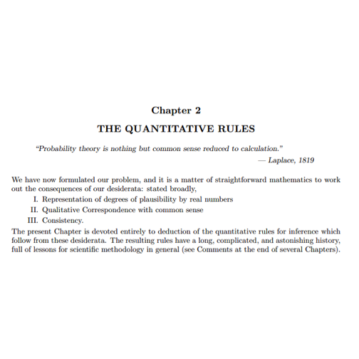
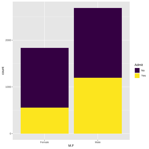
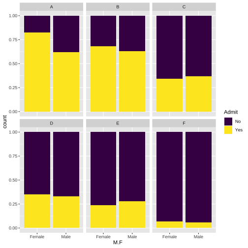
class: center, middle, inverse, title-slide

.title[
# Tidy, Probability and Tables
]
.subtitle[
## The Core of Statistical Thinking
]
.author[
### Robert W. Walker
]
.institute[
### Atkinson Graduate School of Management
]
.date[
### 2023/01/31
]

---

# Tidy thinking

First, how did I import my data?

```r
library(tidyverse)
library(readxl)
Bonds <- read_excel("probtabSMBAP21/data/Week-2.xlsx", sheet = "Bonds")
CEOComp <- read_excel("probtabSMBAP21/data/Week-2.xlsx", sheet = "CEOComp")
FastFood <- read_excel("probtabSMBAP21/data/Week-2.xlsx", sheet = "FastFood", na="NA")
DisabilityExp <- read_excel("probtabSMBAP21/data/Week-2.xlsx", sheet = "DisabilityExp")
UCBAdmit <- read_excel("probtabSMBAP21/data/Week-2.xlsx", sheet = "UCBAdmit")
```

---
# Easier

```r
load(url("https://github.com/robertwwalker/DADMStuff/raw/master/Week3Data.RData"))
```

---
class: inverse, center

# Probability and Tables

---
class: inverse, center

# Probability

![](index_files/figure-html/unnamed-chunk-3-1.png)

---
class: inverse

# Probability

.font150[
Two rules:
1. Probabilities sum to one.
2. The probability of any event is greater than or equal to zero.
]
---
class: inverse

# Where does Probability Come From?

There are three common sources of probabilities:

- Known formula [Dice, Coins, etc.]

- Empirical frequency

- Subjective belief

---
class: inverse

# A priori probability

The probability of a given integer on a k-sided die: `$\frac{1}{k}$`.

The probability of **heads** with a fair coin: `$\frac{1}{2}$`.

The probability of a Queen?  `$\frac{4}{52}$`

The probability of a Diamond?  `$\frac{13}{52}$`

The Queen of Diamonds? `$\frac{1}{52}$` or   `$(\frac{4}{52}\times\frac{13}{52})$`

**Quasirandom numbers**

---
class: inverse

# Empirical probability: frequency

How often does something happen?

[Annie](https://youtu.be/tgC-vZp07YM)

[Straight to Watch](https://www.youtube.com/watch?v=tgC-vZp07YM)

---
class: inverse

# This is Historical Statistics

How likely am I to be admitted? *Consult the admissions rate*

How fast do I drive? *Likelihood of law enforcement and need for speed*

In data: this is tables.

---
# Berkeley

.pull-left[

```
##         
##            No  Yes
##   Female 1278  557
##   Male   1493 1198
```

```
##     M.F   No  Yes
##  Female 1278  557
##    Male 1493 1198
```
]

.pull-right[

```r
library(tidyverse)
library(janitor)
table(UCBAdmit$M.F,UCBAdmit$Admit)
UCBAdmit %>% tabyl(M.F, Admit)
```
]

---
class:inverse

# Three Versions

.pull-left[

```r
prop.table(table(UCBAdmit$M.F,UCBAdmit$Admit), 1)
```

```
##         
##                 No       Yes
##   Female 0.6964578 0.3035422
##   Male   0.5548123 0.4451877
```

```r
prop.table(table(UCBAdmit$M.F,UCBAdmit$Admit), 2)
```

```
##         
##                 No       Yes
##   Female 0.4612053 0.3173789
##   Male   0.5387947 0.6826211
```

```r
prop.table(table(UCBAdmit$M.F,UCBAdmit$Admit))
```

```
##         
##                 No       Yes
##   Female 0.2823685 0.1230667
##   Male   0.3298719 0.2646929
```
]

.pull-right[

```r
UCBAdmit %>% tabyl(M.F, Admit) %>% adorn_percentages("row")
```

```
##     M.F        No       Yes
##  Female 0.6964578 0.3035422
##    Male 0.5548123 0.4451877
```

```r
UCBAdmit %>% tabyl(M.F, Admit) %>% adorn_percentages("col")
```

```
##     M.F        No       Yes
##  Female 0.4612053 0.3173789
##    Male 0.5387947 0.6826211
```

```r
UCBAdmit %>% tabyl(M.F, Admit) %>% adorn_percentages("all")
```

```
##     M.F        No       Yes
##  Female 0.2823685 0.1230667
##    Male 0.3298719 0.2646929
```
]

---
background-image: url("UCBM.png")
background-size: contain
class: bottom

# Plot It

```r
( UCBM <- ggplot(UCBAdmit) + aes(x=M.F, fill=Admit) + geom_bar(position="dodge") + scale_fill_viridis_d() )
```