Human Rights Protections–Tables

Published

February 13, 2023

obertwwalker.github.io

Human Rights Data

Chris Fariss of the University of Michigan has done some very interesting work on human rights protection. You can find tons of stuff on his work on his website. I want to make a table of the data.

Load the Data and Libraries

How’s that done?
library(tidyverse)
library(magrittr)
library(DT)
library(gt)
library(gtExtras)
# install with remotes::install_github("jimjam-slam/ggflags")
library(countrycode)
library(ggflags) 
load("data/HumanRightsProtectionScores_v4.01.Rdata")
HR.Data <- x
rm(x)
HR.Data <- HR.Data %>% left_join(., codelist, by= c("COW" = "cown"))

Let me now put the data into a browseable table.

A Browsable DataTable

This is a panel data structure with two dimensions: countries and years. As a result, though there are not all that many countries in the world, each country is potentially repeated up to 74 times [1946 to 2019]. The filter boxes at the bottom allow you to select ranges of the quantitative indicators.

How’s that done?
HR.Data %<>% 
  mutate(country.name.en = as.factor(country.name.en))
HR.Data %>% 
    arrange(country.name.en, YEAR) %>%
  select(`Country` = country.name.en, `Year` = YEAR, `Human Rights (mean)` = theta_mean, `Human Rights (std. dev.)` = theta_sd, `Killing (mean)` = killing_estimate_mean, `Killing (median)` = killing_estimate_median) %>%
  datatable(., filter = "bottom", extensions = 'Buttons', options = list(
    dom = 'Bfrtip',
    buttons = c('copy', 'csv', 'excel'), 
  initComplete = JS(
    "function(settings, json) {",
    "$(this.api().table().header()).css({'background-color': '#131F4F', 'color': '#fff'});",
    "}")
)) %>%
  formatRound(., 3:6)

A Starter Table

How’s that done?
HR.Summary <- HR.Data %>% 
  group_by(country.name.en) %>% 
  mutate(Obs = n()) %>% 
  filter(Obs==74) %>% 
  summarise(Obs = mean(Obs), 
            Mean = mean(theta_mean, na.rm=TRUE), 
            SD = sd(theta_mean)
            )
HR.Summary %>% mutate(Country = country.name.en) %>%
  select(-country.name.en) %>% 
  relocate(Country, .before=Obs) %>% 
  gt() %>%
  cols_label(SD = "Std. Dev.")
Country Obs Mean Std. Dev.
Afghanistan 74 -0.808239676 1.5835807
Albania 74 -0.733855668 1.1318765
Argentina 74 -0.109687027 0.8659722
Australia 74 1.496089393 0.4821145
Austria 74 1.363463386 0.7163969
Belgium 74 1.950358681 0.8702604
Bhutan 74 1.639800956 0.8947993
Bolivia 74 0.031485088 0.6004716
Brazil 74 -0.986771401 0.4380970
Bulgaria 74 -0.141004868 0.8164432
Canada 74 1.513579623 1.0867982
Chile 74 -0.116312712 1.0980581
China 74 -1.690418324 0.5866867
Colombia 74 -1.549160011 0.3371290
Costa Rica 74 1.407450473 0.5889534
Cuba 74 -0.780236659 0.6767858
Czechia 74 0.234391962 1.7996961
Denmark 74 2.408907458 0.7988521
Dominican Republic 74 -0.353273333 0.4778804
Ecuador 74 -0.065637090 0.4093959
Egypt 74 -0.953780511 0.3387420
El Salvador 74 -0.456976650 1.0261214
Ethiopia 74 -1.250759418 0.9343362
Finland 74 2.234185764 0.9850571
France 74 0.732780358 0.7610454
Greece 74 0.343929239 0.6769572
Guatemala 74 -1.243405610 1.0571324
Haiti 74 -0.700733551 0.7827763
Honduras 74 -0.004659247 0.6012447
Hungary 74 0.316610321 1.1781173
Iceland 74 4.448582351 0.7721095
Iran 74 -1.490454238 0.5933340
Iraq 74 -1.759200305 0.6444676
Ireland 74 1.714516245 0.8303707
Italy 74 0.747846387 0.5781654
Japan 74 1.346933187 0.8414272
Jordan 74 -0.167098074 0.3324552
Lebanon 74 -0.501174232 0.5096649
Liberia 74 0.016102174 0.9964066
Luxembourg 74 4.610048247 0.7513979
Mexico 74 -0.698399686 0.4417479
Mongolia 74 1.979956542 0.8973234
Nepal 74 -0.407058523 0.7314475
Netherlands 74 2.179110741 1.6230486
New Zealand 74 3.388201387 0.5058292
Nicaragua 74 -0.334761828 0.8095413
Norway 74 2.580217186 1.2412017
Oman 74 1.083276811 0.4880672
Panama 74 0.534798448 0.9244702
Paraguay 74 -0.431996166 0.8683609
Peru 74 -0.398071785 0.8472583
Philippines 74 -1.442899788 0.5619596
Poland 74 0.228957535 1.2563224
Portugal 74 0.513038978 1.4489625
Romania 74 -0.552472696 0.9883813
Russia 74 -1.596063064 0.3926173
Saudi Arabia 74 -0.087345053 0.4736322
South Africa 74 -1.013630691 0.5891013
Spain 74 0.389802441 0.7055324
Sweden 74 1.675085472 1.0897249
Switzerland 74 1.177549367 0.8326230
Syria 74 -1.051481698 0.6846712
Thailand 74 -0.511999725 0.4080301
Turkey 74 -0.890056818 0.4962535
United Kingdom 74 0.890858555 0.8947926
United States 74 0.232456052 1.2330506
Uruguay 74 0.649137406 1.4119239
Venezuela 74 -0.585731862 0.7032445

Improving the Table

I want to add some things to this. I want a spanning header for the three bits of actual human rights data that I am using. I also want a list column of the data to feed to the sparkline function to generate the time series plot. I found a file of flags on my hard drive that I got from somewhere and I want to deploy them in the table. I will also round the digits

How’s that done?
library(countrycode)
Flags <- read.csv("data/flags_iso.csv")
HR.Summary <- HR.Data %>% 
  group_by(country.name.en) %>% 
  mutate(Obs = n()) %>% 
  filter(Obs==74) %>%
  arrange(YEAR) %>%
  summarise(Obs = mean(Obs), 
            Mean = mean(theta_mean, na.rm=TRUE), 
            SD = sd(theta_mean), 
            hr_data = list(theta_mean),
            .groups = "drop")
CCs <- codelist %>% select(country.name.en, iso3c)
HR.Summary <- HR.Summary %>% 
  left_join(., CCs) %>%
  left_join(., Flags, 
            by=c("iso3c" = "Alpha.3.code")) %>%
  select(-iso3c, -Country, -Alpha.2.code) %>%
  relocate(., URL, .after=country.name.en)
My.Table <- HR.Summary %>%
  gt() %>%
# format the numeric output to 3 digit rounding  
  fmt_number(columns = c(Mean, SD),
             decimals = 3) %>%
# create nice labels for a few ugly variable names
  cols_label(country.name.en = "Country",
             SD = "Std. Dev.",
             hr_data = "Time Series Plot",
             URL = "Flag") %>%
# Plot the sparklines from the list column
  gt_plt_sparkline(hr_data, 
                   type="ref_median", 
                   same_limit = TRUE
                   ) %>%
# Plot the flags from the included URL's in the data
  gt_img_rows(URL, img_source = "web", height = 30) %>%
# use the guardian's table theme
  gt_theme_guardian() %>% 
# give hulk coloring to the Mean Human Rights Score
  gt_hulk_col_numeric(Mean) %>%
# create a header and subheader
  tab_header(title="Human Rights Data Summary", subtitle = "Data from Fariss (2020)") %>%
# create the spanner heading
  tab_spanner(label = "Human Rights Measures",
    columns = c(
      Mean, SD, hr_data)
    )
# save the original as an image
gtsave(My.Table, "Table.png")
# show the table themed in accordance with the page
My.Table
Human Rights Data Summary Data from Fariss (2020) Country Flag Obs Human Rights Measures Mean Std. Dev. Time Series Plot Afghanistan 74 −0.808 1.584 Albania 74 −0.734 1.132 Argentina 74 −0.110 0.866 Australia 74 1.496 0.482 Austria 74 1.363 0.716 Belgium 74 1.950 0.870 Bhutan 74 1.640 0.895 Bolivia 74 0.031 0.600 Brazil 74 −0.987 0.438 Bulgaria 74 −0.141 0.816 Canada 74 1.514 1.087 Chile 74 −0.116 1.098 China 74 −1.690 0.587 Colombia 74 −1.549 0.337 Costa Rica 74 1.407 0.589 Cuba 74 −0.780 0.677 Czechia 74 0.234 1.800 Denmark 74 2.409 0.799 Dominican Republic 74 −0.353 0.478 Ecuador 74 −0.066 0.409 Egypt 74 −0.954 0.339 El Salvador 74 −0.457 1.026 Ethiopia 74 −1.251 0.934 Finland 74 2.234 0.985 France 74 0.733 0.761 Greece 74 0.344 0.677 Guatemala 74 −1.243 1.057 Haiti 74 −0.701 0.783 Honduras 74 −0.005 0.601 Hungary 74 0.317 1.178 Iceland 74 4.449 0.772 Iran 74 −1.490 0.593 Iraq 74 −1.759 0.644 Ireland 74 1.715 0.830 Italy 74 0.748 0.578 Japan 74 1.347 0.841 Jordan 74 −0.167 0.332 Lebanon 74 −0.501 0.510 Liberia 74 0.016 0.996 Luxembourg 74 4.610 0.751 Mexico 74 −0.698 0.442 Mongolia 74 1.980 0.897 Nepal 74 −0.407 0.731 Netherlands 74 2.179 1.623 New Zealand 74 3.388 0.506 Nicaragua 74 −0.335 0.810 Norway 74 2.580 1.241 Oman 74 1.083 0.488 Panama 74 0.535 0.924 Paraguay 74 −0.432 0.868 Peru 74 −0.398 0.847 Philippines 74 −1.443 0.562 Poland 74 0.229 1.256 Portugal 74 0.513 1.449 Romania 74 −0.552 0.988 Russia 74 −1.596 0.393 Saudi Arabia 74 −0.087 0.474 South Africa 74 −1.014 0.589 Spain 74 0.390 0.706 Sweden 74 1.675 1.090 Switzerland 74 1.178 0.833 Syria 74 −1.051 0.685 Thailand 74 −0.512 0.408 Turkey 74 −0.890 0.496 United Kingdom 74 0.891 0.895 United States 74 0.232 1.233 Uruguay 74 0.649 1.412 Venezuela 74 −0.586 0.703

Image of Table

References

How’s that done?
knitr::write_bib(names(sessionInfo()$otherPkgs), file="bibliography.bib")

References

Arel-Bundock, Vincent. 2022. Countrycode: Convert Country Names and Country Codes. https://vincentarelbundock.github.io/countrycode/.
Arel-Bundock, Vincent, Nils Enevoldsen, and CJ Yetman. 2018. “Countrycode: An r Package to Convert Country Names and Country Codes.” Journal of Open Source Software 3 (28): 848. https://doi.org/10.21105/joss.00848.
Auguie, Baptiste. 2023. Ggflags: Plot Flags of the World in Ggplot2.
Bache, Stefan Milton, and Hadley Wickham. 2022. Magrittr: A Forward-Pipe Operator for r. https://CRAN.R-project.org/package=magrittr.
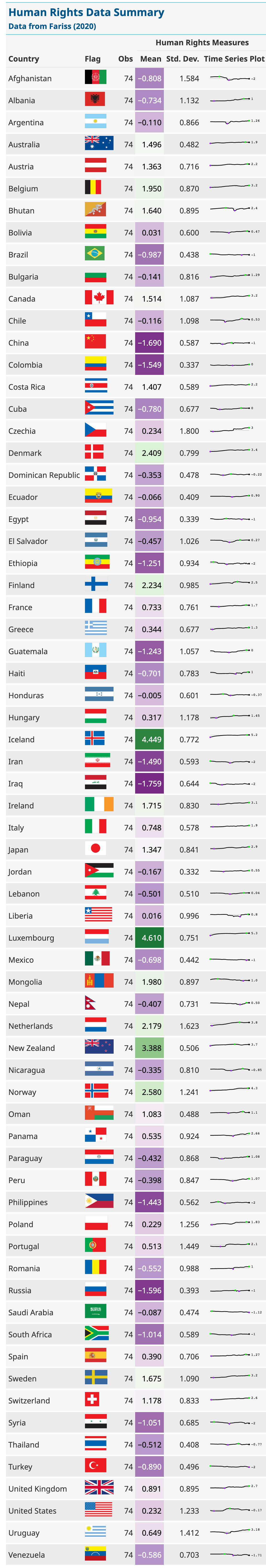
Fariss, Christopher, Michael Kenwick, and Kevin Reuning. 2020. Latent Human Rights Protection Scores Version 4.” Harvard Dataverse. https://doi.org/10.7910/DVN/RQ85GK.
Iannone, Richard, Joe Cheng, Barret Schloerke, Ellis Hughes, and JooYoung Seo. 2022. Gt: Easily Create Presentation-Ready Display Tables. https://CRAN.R-project.org/package=gt.
Mock, Thomas. 2022. gtExtras: Extending Gt for Beautiful HTML Tables. https://CRAN.R-project.org/package=gtExtras.
Müller, Kirill, and Hadley Wickham. 2022. Tibble: Simple Data Frames. https://CRAN.R-project.org/package=tibble.
Wickham, Hadley. 2016. Ggplot2: Elegant Graphics for Data Analysis. Springer-Verlag New York. https://ggplot2.tidyverse.org.
———. 2022a. Stringr: Simple, Consistent Wrappers for Common String Operations. https://CRAN.R-project.org/package=stringr.
———. 2022b. Tidyverse: Easily Install and Load the Tidyverse. https://CRAN.R-project.org/package=tidyverse.
———. 2023. Forcats: Tools for Working with Categorical Variables (Factors). https://CRAN.R-project.org/package=forcats.
Wickham, Hadley, Mara Averick, Jennifer Bryan, Winston Chang, Lucy D’Agostino McGowan, Romain François, Garrett Grolemund, et al. 2019. “Welcome to the tidyverse.” Journal of Open Source Software 4 (43): 1686. https://doi.org/10.21105/joss.01686.
Wickham, Hadley, Winston Chang, Lionel Henry, Thomas Lin Pedersen, Kohske Takahashi, Claus Wilke, Kara Woo, Hiroaki Yutani, and Dewey Dunnington. 2022. Ggplot2: Create Elegant Data Visualisations Using the Grammar of Graphics. https://CRAN.R-project.org/package=ggplot2.
Wickham, Hadley, Romain François, Lionel Henry, Kirill Müller, and Davis Vaughan. 2023. Dplyr: A Grammar of Data Manipulation. https://CRAN.R-project.org/package=dplyr.
Wickham, Hadley, and Lionel Henry. 2023. Purrr: Functional Programming Tools. https://CRAN.R-project.org/package=purrr.
Wickham, Hadley, Jim Hester, and Jennifer Bryan. 2022. Readr: Read Rectangular Text Data. https://CRAN.R-project.org/package=readr.
Wickham, Hadley, Davis Vaughan, and Maximilian Girlich. 2023. Tidyr: Tidy Messy Data. https://CRAN.R-project.org/package=tidyr.
Xie, Yihui, Joe Cheng, and Xianying Tan. 2023. DT: A Wrapper of the JavaScript Library DataTables. https://github.com/rstudio/DT.