How’s that done?
library(plumber)
knitr::write_bib(names(sessionInfo()$otherPkgs), file="bibliography.bib")In his talk at rstudio::conf, Joe Cheng discussed the arrival of shinylive for R. Coming almost a year after the python deployment, it is really nice to think about teaching it and not having to teach computer science but it would have to reliably work for that dream to become reality. So I decided to try it out.
Take an app and try to build it into shinylive. It works.
Here is my app. I do not know where it originally came from – the data that is – but it is very simple.
# Forecasting Google ----
# It supports 3 stats forecasting models - Linear Regression, ARIMA, and Holt-Winters
library(shiny)
GOOG <- [data downloaded via tq_get in tidyquant and turned into a daily ts object, check the repo for the actual data]
# UI ----
ui <- fluidPage(
# App title ----
titlePanel("Forecasting Sandbox"),
sidebarLayout(
sidebarPanel(width = 3,
selectInput(inputId = "model",
label = "Select Model",
choices = c("Linear Regression", "ARIMA", "Holt-Winters"),
selected = "Linear Regression"),
# Linear Regression model arguments
conditionalPanel(condition = "input.model == 'Linear Regression'",
checkboxGroupInput(inputId = "lm_args",
label = "Select Regression Features:",
choices = list("Trend" = 1,
"Seasonality" = 2),
selected = 1)),
# ARIMA model arguments
conditionalPanel(condition = "input.model == 'ARIMA'",
h5("Order Parameters"),
sliderInput(inputId = "p",
label = "p:",
min = 0,
max = 5,
value = 0),
sliderInput(inputId = "d",
label = "d:",
min = 0,
max = 5,
value = 0),
sliderInput(inputId = "q",
label = "q:",
min = 0,
max = 5,
value = 0),
h5("Seasonal Parameters:"),
sliderInput(inputId = "P",
label = "P:",
min = 0,
max = 5,
value = 0),
sliderInput(inputId = "D",
label = "D:",
min = 0,
max = 5,
value = 0),
sliderInput(inputId = "Q",
label = "Q:",
min = 0,
max = 5,
value = 0)
),
# Holt Winters model arguments
conditionalPanel(condition = "input.model == 'Holt-Winters'",
checkboxGroupInput(inputId = "hw_args",
label = "Select Holt-Winters Parameters:",
choices = list("Beta" = 2,
"Gamma" = 3),
selected = c(1, 2, 3)),
selectInput(inputId = "hw_seasonal",
label = "Select Seasonal Type:",
choices = c("Additive", "Multiplicative"),
selected = "Additive")),
checkboxInput(inputId = "log",
label = "Log Transformation",
value = FALSE),
sliderInput(inputId = "h",
label = "Forecasting Horizon:",
min = 1,
max = 60,
value = 24)
# actionButton(inputId = "update",
# label = "Update!")
),
# Main panel for displaying outputs ----
mainPanel(width = 9,
# Forecast Plot ----
plotOutput(outputId = "fc_plot",
height = "400px")
)
)
)
# Define server logic required to draw a histogram ----
server <- function(input, output) {
# Load the dataset a reactive object
d <- reactiveValues(df = data.frame(input = as.numeric(GOOG),
index = seq.Date(from= as.Date("2016-05-19"),
by = "day",
length.out = length(GOOG))),
air = GOOG)
# Log transformation
observeEvent(input$log,{
if(input$log){
d$df <- data.frame(input = log(as.numeric(GOOG)),
index = seq.Date(from = as.Date("2016-05-19"),
by = "day",
length.out = length(GOOG)))
d$air <- log(GOOG)
} else {
d$df <- data.frame(input = as.numeric(GOOG),
index = seq.Date(from = as.Date("2016-05-19"),
by = "day",
length.out = length(GOOG)))
d$air <- GOOG
}
})
# The forecasting models execute under the plot render
output$fc_plot <- renderPlot({
# if adding a prediction intervals level argument set over here
pi <- 0.95
# Holt-Winters model
if(input$model == "Holt-Winters"){
a <- b <- c <- NULL
if(!"2" %in% input$hw_args){
b <- FALSE
}
if(!"3" %in% input$hw_args){
c <- FALSE
}
md <- HoltWinters(d$air,
seasonal = ifelse(input$hw_seasonal == "Additive", "additive", "multiplicative"),
beta = b,
gamma = c
)
fc <- predict(md, n.ahead = input$h, prediction.interval = TRUE) |>
as.data.frame()
fc$index <- seq.Date(from = as.Date(Sys.Date()),
by = "day",
length.out = input$h)
# ARIMA model
} else if(input$model == "ARIMA"){
md <- arima(d$air,
order = c(input$p, input$d, input$q),
seasonal = list(order = c(input$P, input$D, input$Q))
)
fc <- predict(md, n.ahead = input$h, prediction.interval = TRUE) |>
as.data.frame()
names(fc) <- c("fit", "se")
fc$index <- seq.Date(from = as.Date(Sys.Date()),
by = "day",
length.out = input$h)
fc$upr <- fc$fit + 1.96 * fc$se
fc$lwr <- fc$fit - 1.96 * fc$se
# Linear Regression model
} else if(input$model == "Linear Regression"){
d_lm <- d$df
d_fc <- data.frame(index = seq.Date(from = as.Date(Sys.Date()),
by = "day",
length.out = input$h))
if("1" %in% input$lm_args){
d_lm$trend <- 1:nrow(d_lm)
d_fc$trend <- (max(d_lm$trend) + 1):(max(d_lm$trend) + input$h)
}
if("2" %in% input$lm_args){
d_lm$season <- as.factor(months((d_lm$index)))
d_fc$season <- factor(months((d_fc$index)), levels = levels(d_lm$season))
}
md <- lm(input ~ ., data = d_lm[, - which(names(d_lm) == "index")])
fc <- predict(md, n.ahead = input$h, interval = "prediction",
level = pi, newdata = d_fc) |>
as.data.frame()
fc$index <- seq.Date(from = as.Date(Sys.Date()),
by = "day",
length.out = input$h)
}
# Setting the plot
at_x <- pretty(seq.Date(from = min(d$df$index),
to = max(fc$index),
by = "day"))
at_y <- c(pretty(c(d$df$input, fc$upr)), 60)
plot(x = d$df$index, y = d$df$input,
col = "#1f77b4",
type = "l",
frame.plot = FALSE,
axes = FALSE,
panel.first = abline(h = at_y, col = "grey80"),
main = "GOOG Forecast",
xlim = c(min(d$df$index), max(fc$index)),
ylim = c(min(c(min(d$df$input), min(fc$lwr))), max(c(max(fc$upr), max(d$df$input)))),
xlab = paste("Model:", input$model, sep = " "),
ylab = "GOOG Price")
mtext(side =1, text = format(at_x, format = "%Y-%M"), at = at_x,
col = "grey20", line = 1, cex = 0.8)
mtext(side =2, text = format(at_y, scientific = FALSE), at = at_y,
col = "grey20", line = 1, cex = 0.8)
lines(x = fc$index, y = fc$fit, col = '#1f77b4', lty = 2, lwd = 2)
lines(x = fc$index, y = fc$upr, col = 'blue', lty = 2, lwd = 2)
lines(x = fc$index, y = fc$lwr, col = 'blue', lty = 2, lwd = 2)
})
}
# Create Shiny app ----
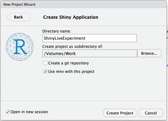
shinyApp(ui = ui, server = server)The first step is to start a new shiny project. For this one, I will use renv as the documents suggest this to be useful. The New project dialog can be used to accomplish nearly all of this.
Ok. Now there is a shiny app in a directory to use. Now let’s try the shinylive package.
install.packages("shinylive")In theory, there is not that much to it so long as the app works with webR. So let’s compile it up and see what happens. There is an app.R file in myapp and that becomes the docs directory when transformed by shiny live. This all exists in a repository called SLT2 that can be found here. At first, I wanted to put it as a subdirectory here but could not quite get it all to render properly. With the separate repo, building the app in docs means that github pages can render it.
shinylive::export(appdir = "myapp", outputdir = "docs")
If it works, the docs directory of that repository has a forecasting app. I serve it using github pages.
library(plumber)
knitr::write_bib(names(sessionInfo()$otherPkgs), file="bibliography.bib")