ARCH Models: Blair Approval Rating

panel data
code
analysis
Author

Robert W. Walker

Published

July 24, 2026

Introduction

Overview

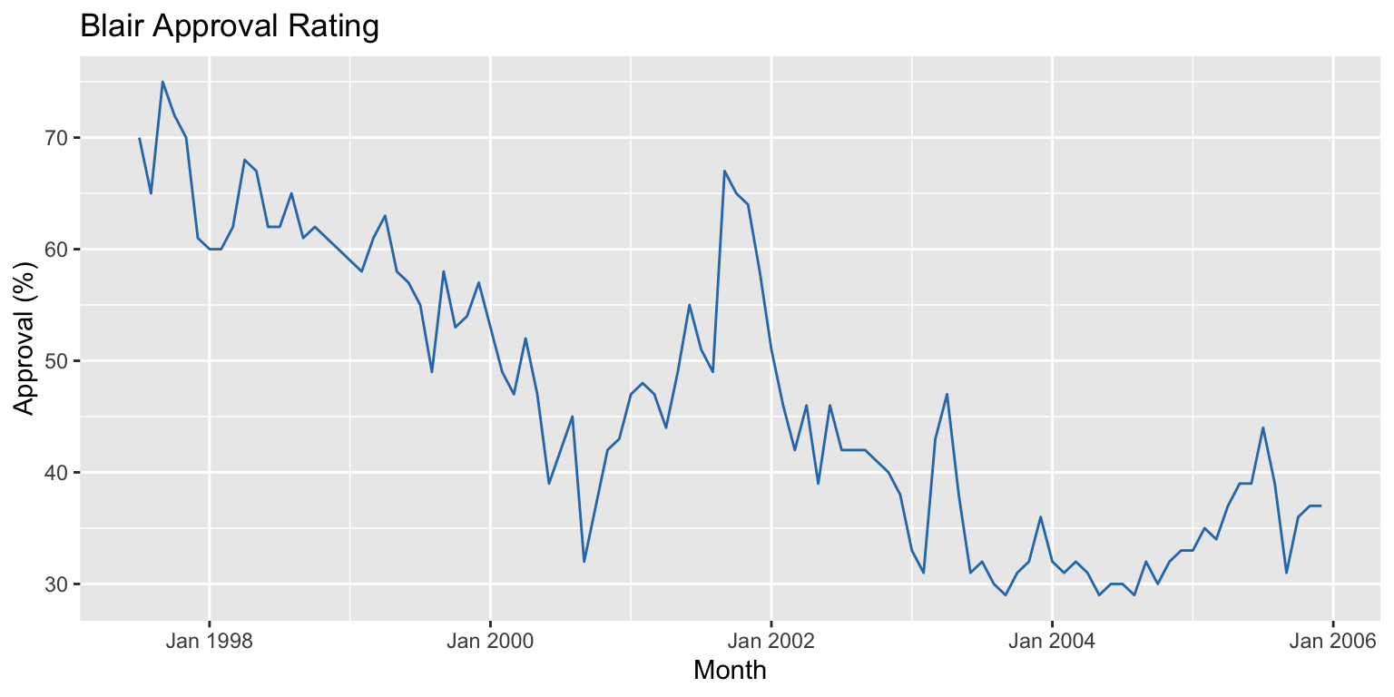
This document works through an ARCH modelling example using Tony Blair’s monthly approval ratings from June 1997 onward. Each section presents R and Stata tabs side by side. The R tab is executed and results are shown on the page; the Stata tab provides equivalent syntax for reference. It extends the ECM analysis to ARCH.

Variables in tonyapp4.dta:

Variable Description
app Blair approval rating (%)
labecman % thinking Labour best manager of the economy
v911d 9/11 dummy (pre-stored, already differenced)
petrold Petrol crisis dummy (pre-stored, differenced)
casl Iraq casualties (logged)
casld Iraq casualties logged, differenced
appd app, first-differenced (pre-stored)
labecmand labecman, first-differenced (pre-stored)
v911 9/11 dummy (raw, for differencing)
petrol Petrol crisis dummy (raw, for differencing)

1. Setup

library(haven)     # read .dta files
library(zoo)       # yearmon monthly time index

Attaching package: 'zoo'
The following objects are masked from 'package:base':

    as.Date, as.Date.numeric
library(urca)      # ur.df  (Dickey-Fuller — matches Stata's dfuller)
library(fracdiff)  # fracdiff  (ARFIMA models)
library(rugarch)   # ugarchspec / ugarchfit  (ARCH/GARCH)
Loading required package: parallel
library(ggplot2)   # plotting
* All procedures used here are built into Stata.
* No package installation is required.

2. Load Data

df <- read_dta("./data/tonyapp4.dta")
cd "C:\icpsrdyn\Lab"
use "tonyapp4.dta", clear

3. Create Monthly Time Index

Stata’s %tm format counts months from January 1960 (month 0). The counter variable runs 0, 1, 2, … and month = counter + 450. Since month 0 = Jan 1960 and 12 × 37 + 6 = 450, month 450 = July 1997. (The .do file comment says “June” but the Stata log confirms 1997m7 to 2005m12.) In R we use zoo::yearmon.

n          <- nrow(df)
df$counter <- 0:(n - 1)

# month 450 in Stata %tm = July 1997 (not June — see note above)
df$month   <- as.yearmon("1997-07") + df$counter / 12
* counter = 0, 1, 2, … ; month 450 in %tm = July 1997
egen counter = fill(0 1 2 3)
gen  month   = counter + 450
format month %tm
tsset month
* Stata confirms: Time variable: month, 1997m7 to 2005m12

4. Blair Approval Rating

4.1 Exploratory Plot

ggplot(df, aes(x = month, y = app)) +
  geom_line(colour = "#2c7bb6") +
  labs(title = "Blair Approval Rating",
       x = "Month", y = "Approval (%)")

label variable app "Blair Approval Rating"
twoway line app month

4.2 Stationarity Tests (Dickey-Fuller)

Stata’s dfuller defaults to 0 augmentation lags, no constant, and no trend (H₀: random walk without drift). urca::ur.df() with type = "none" and lags = 0 matches this specification exactly. tseries::adf.test() — which auto-selects lags and includes both a constant and trend — produces notably different statistics and should be avoided for direct comparison.

# type="none": no constant, no trend — matches Stata's dfuller default
# lags=0: no augmentation — matches Stata's "Number of lags = 0"
summary(ur.df(df$app,        type = "none", lags = 0))   # level

############################################### 
# Augmented Dickey-Fuller Test Unit Root Test # 
############################################### 

Test regression none 


Call:
lm(formula = z.diff ~ z.lag.1 - 1)

Residuals:
     Min       1Q   Median       3Q      Max 
-12.4602  -2.4362  -0.2563   2.7197  18.5878 

Coefficients:
         Estimate Std. Error t value Pr(>|t|)
z.lag.1 -0.011995   0.009446   -1.27    0.207

Residual standard error: 4.595 on 100 degrees of freedom
Multiple R-squared:  0.01587,   Adjusted R-squared:  0.006029 
F-statistic: 1.613 on 1 and 100 DF,  p-value: 0.2071


Value of test-statistic is: -1.2699 

Critical values for test statistics: 
      1pct  5pct 10pct
tau1 -2.58 -1.95 -1.62
summary(ur.df(diff(df$app),  type = "none", lags = 0))   # first difference

############################################### 
# Augmented Dickey-Fuller Test Unit Root Test # 
############################################### 

Test regression none 


Call:
lm(formula = z.diff ~ z.lag.1 - 1)

Residuals:
     Min       1Q   Median       3Q      Max 
-12.6322  -2.7404  -0.6839   2.1063  17.7548 

Coefficients:
        Estimate Std. Error t value Pr(>|t|)    
z.lag.1 -1.12261    0.09915  -11.32   <2e-16 ***
---
Signif. codes:  0 '***' 0.001 '**' 0.01 '*' 0.05 '.' 0.1 ' ' 1

Residual standard error: 4.592 on 99 degrees of freedom
Multiple R-squared:  0.5642,    Adjusted R-squared:  0.5598 
F-statistic: 128.2 on 1 and 99 DF,  p-value: < 2.2e-16


Value of test-statistic is: -11.3219 

Critical values for test statistics: 
      1pct  5pct 10pct
tau1 -2.58 -1.95 -1.62
dfuller app      /* Z(t) = -2.262,  p = 0.1847 */
dfuller d.app    /* Z(t) = -11.314, p = 0.0000 */

5. ARFIMA Models

Warning

Estimation method mismatch — R and Stata will differ here.
Stata’s arfima uses exact maximum likelihood. fracdiff::fracdiff() uses the Haslett–Raftery (1989) spectral approximation, which for these data finds d ≈ 0 (no evidence of fractional integration). Stata’s exact MLE finds d ≈ −0.28 (significant at 1%), implying mild overdifferencing. The qualitative conclusion depends on the estimator.
For R results closer to Stata, consider forecast::arfima(dapp, estim = "mle").

dapp <- diff(df$app)

# ARFIMA(0, d, 0) — Stata finds d = -0.278 (SE 0.092, z = -3.01, p = 0.003)
fracdiff(dapp)

Call:
  fracdiff(x = dapp) 

Coefficients:
           d 
4.583013e-05 
sigma[eps] = 4.596884 
a list with components:
 [1] "log.likelihood"  "n"               "msg"             "d"              
 [5] "ar"              "ma"              "covariance.dpq"  "fnormMin"       
 [9] "sigma"           "stderror.dpq"    "correlation.dpq" "h"              
[13] "d.tol"           "M"               "hessian.dpq"     "length.w"       
[17] "residuals"       "fitted"          "call"           
# ARFIMA(1, d, 0) — Stata finds d = -0.474, ar = 0.253
fracdiff(dapp, nar = 1)
Warning: unable to compute correlation matrix; maybe change 'h'

Call:
  fracdiff(x = dapp, nar = 1) 

*** Warning during (fdcov) fit: unable to compute correlation matrix; maybe change 'h'

Coefficients:
            d            ar 
 4.583013e-05 -1.276140e-01 
sigma[eps] = 4.581019 
a list with components:
 [1] "log.likelihood"  "n"               "msg"             "d"              
 [5] "ar"              "ma"              "covariance.dpq"  "fnormMin"       
 [9] "sigma"           "stderror.dpq"    "correlation.dpq" "h"              
[13] "d.tol"           "M"               "hessian.dpq"     "length.w"       
[17] "residuals"       "fitted"          "call"           
arfima d.app              /* d = -0.278, SE 0.092, z = -3.01, p = 0.003 */
arfima d.app, ar(1)       /* d = -0.474, ar(1) = 0.253                  */

ARFIMA with external regressors — Stata accepts xreg directly; fracdiff does not, so we pre-filter first:

# Pre-filter: partial out d.v911 and d.petrol before estimating d
dv911   <- diff(df$v911)
dpetrol <- diff(df$petrol)
pre_fit <- lm(dapp ~ dv911 + dpetrol)

# ARFIMA(0, d, 1) on residuals — approximate equivalent
# Stata finds: d.v911=10.61, d.petrol=-9.01, d=-0.470, ma(1)=0.339
fracdiff(residuals(pre_fit), nma = 1)
Warning: unable to compute correlation matrix; maybe change 'h'

Call:
  fracdiff(x = residuals(pre_fit), nma = 1) 

*** Warning during (fdcov) fit: unable to compute correlation matrix; maybe change 'h'

Coefficients:
           d           ma 
4.583013e-05 6.353972e-02 
sigma[eps] = 4.200936 
a list with components:
 [1] "log.likelihood"  "n"               "msg"             "d"              
 [5] "ar"              "ma"              "covariance.dpq"  "fnormMin"       
 [9] "sigma"           "stderror.dpq"    "correlation.dpq" "h"              
[13] "d.tol"           "M"               "hessian.dpq"     "length.w"       
[17] "residuals"       "fitted"          "call"           
/* d.v911=10.607, d.petrol=-9.007, d=-0.470, ma(1)=0.339 */
arfima d.app d.v911 d.petrol, ma(1)

6. Labour Economic Management

6.1 Stationarity Tests

summary(ur.df(df$labecman,       type = "none", lags = 0))   # level

############################################### 
# Augmented Dickey-Fuller Test Unit Root Test # 
############################################### 

Test regression none 


Call:
lm(formula = z.diff ~ z.lag.1 - 1)

Residuals:
     Min       1Q   Median       3Q      Max 
-14.4701  -1.2809   0.6056   2.8108  11.8326 

Coefficients:
        Estimate Std. Error t value Pr(>|t|)
z.lag.1 -0.03785    0.02418  -1.565    0.121

Residual standard error: 4.183 on 100 degrees of freedom
Multiple R-squared:  0.02392,   Adjusted R-squared:  0.01416 
F-statistic:  2.45 on 1 and 100 DF,  p-value: 0.1207


Value of test-statistic is: -1.5653 

Critical values for test statistics: 
      1pct  5pct 10pct
tau1 -2.58 -1.95 -1.62
summary(ur.df(diff(df$labecman), type = "none", lags = 0))   # first difference

############################################### 
# Augmented Dickey-Fuller Test Unit Root Test # 
############################################### 

Test regression none 


Call:
lm(formula = z.diff ~ z.lag.1 - 1)

Residuals:
    Min      1Q  Median      3Q     Max 
-14.482  -1.974   0.000   2.574  10.353 

Coefficients:
        Estimate Std. Error t value Pr(>|t|)    
z.lag.1 -1.12939    0.09895  -11.41   <2e-16 ***
---
Signif. codes:  0 '***' 0.001 '**' 0.01 '*' 0.05 '.' 0.1 ' ' 1

Residual standard error: 4.19 on 99 degrees of freedom
Multiple R-squared:  0.5682,    Adjusted R-squared:  0.5638 
F-statistic: 130.3 on 1 and 99 DF,  p-value: < 2.2e-16


Value of test-statistic is: -11.4138 

Critical values for test statistics: 
      1pct  5pct 10pct
tau1 -2.58 -1.95 -1.62
label variable labecman "Labour Best Eco Mng"
dfuller labecman    /* Z(t) = -2.380, p = 0.1474 */
dfuller d.labecman  /* Z(t) = -11.359, p = 0.0000 */

6.2 Overlay Plot

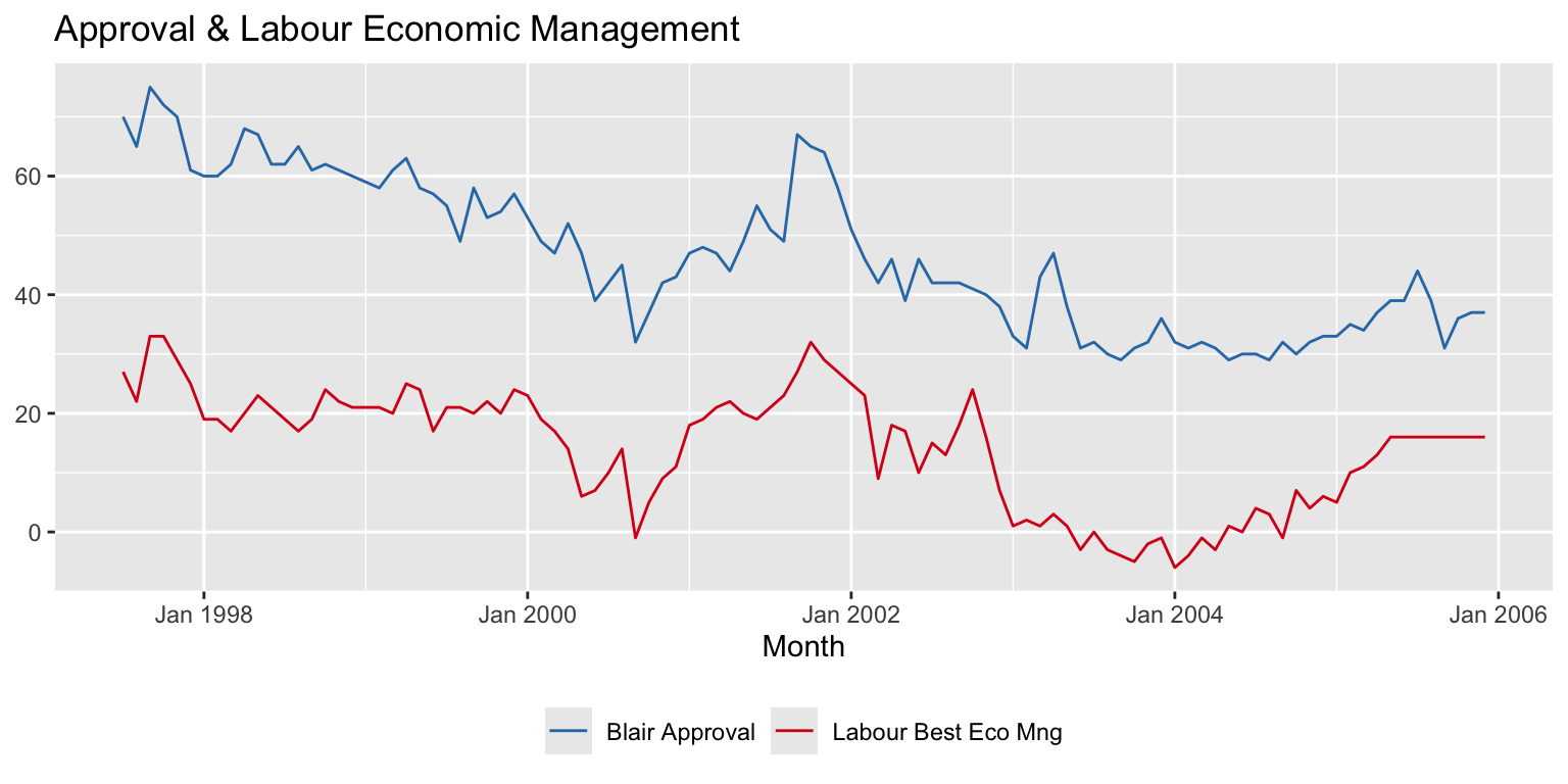
Both series appear non-stationary; plotting together to inspect potential cointegration.

ggplot(df, aes(x = month)) +
  geom_line(aes(y = app,      colour = "Blair Approval")) +
  geom_line(aes(y = labecman, colour = "Labour Best Eco Mng")) +
  scale_colour_manual(
    values = c("Blair Approval"      = "#2c7bb6",
               "Labour Best Eco Mng" = "#d7191c")
  ) +
  labs(title  = "Approval & Labour Economic Management",
       x = "Month", y = NULL, colour = NULL) +
  theme(legend.position = "bottom")

twoway line app month || line labecman month

6.3 Cointegration Residuals (Engle-Granger)

Regress app on labecman; if the residuals are I(0), the two series are cointegrated. The lag choice matters critically here: with 4 lags (the adf.test() default) R fails to reject the unit root (p ≈ 0.34), while Stata with 0 lags rejects at 1% (p = 0.0025). Using ur.df with lags = 0 aligns the test with Stata.

reg_coint       <- lm(app ~ labecman, data = df)
df$ecm_labecman <- residuals(reg_coint)

# With lags=0 (matching dfuller): test stat ≈ -3.84, critical value 1% = -2.60
# → reject unit root → cointegration supported (matches Stata)
summary(ur.df(df$ecm_labecman, type = "none", lags = 0))

############################################### 
# Augmented Dickey-Fuller Test Unit Root Test # 
############################################### 

Test regression none 


Call:
lm(formula = z.diff ~ z.lag.1 - 1)

Residuals:
     Min       1Q   Median       3Q      Max 
-10.5428  -3.4681  -0.8156   2.7531  12.3382 

Coefficients:
        Estimate Std. Error t value Pr(>|t|)    
z.lag.1 -0.26380    0.06832  -3.861    2e-04 ***
---
Signif. codes:  0 '***' 0.001 '**' 0.01 '*' 0.05 '.' 0.1 ' ' 1

Residual standard error: 4.742 on 100 degrees of freedom
Multiple R-squared:  0.1298,    Adjusted R-squared:  0.121 
F-statistic: 14.91 on 1 and 100 DF,  p-value: 0.0002002


Value of test-statistic is: -3.8613 

Critical values for test statistics: 
      1pct  5pct 10pct
tau1 -2.58 -1.95 -1.62
reg app labecman
predict ecm_labecman, resid
dfuller ecm_labecman   /* Z(t) = -3.838, p = 0.0025 → cointegrated */

7. Error Correction Model (OLS)

The ECM takes d.app as dependent variable. L.app and L.labecman provide the error-correction terms.

7.1 Construct Lag and Difference Variables

Stata resolves d., L., and L2D. operators on the fly. In R we build them explicitly.

df$dapp       <- c(NA, diff(df$app))
df$dlabecman  <- c(NA, diff(df$labecman))
df$L_app      <- c(NA, head(df$app,      -1))
df$L_labecman <- c(NA, head(df$labecman, -1))

# L2D.casl = second lag of first difference of casl
dcasl      <- c(NA, diff(df$casl))
df$L2Dcasl <- c(NA, NA, head(dcasl, -2))

# L.casl = one-period lag of casl (used in ARCH variance equation)
df$L_casl  <- c(NA, head(df$casl, -1))
* Stata resolves d.app, L.app, L2D.casl, etc. automatically at estimation time.
label var v911d   "911 differenced"
label var petrold "Petrol Crisis differenced"
label var casld   "Iraq casualties Logged differenced"
label var casl    "Iraq casualties Logged"

7.2 OLS Regression

OLS coefficients match Stata to 4–5 significant figures — no rounding issues here.

reg_ecm <- lm(dapp ~ dlabecman + L_app + L_labecman +
                v911d + petrold + L2Dcasl,
              data = df)
summary(reg_ecm)

Call:
lm(formula = dapp ~ dlabecman + L_app + L_labecman + v911d + 
    petrold + L2Dcasl, data = df)

Residuals:
   Min     1Q Median     3Q    Max 
-9.035 -2.336 -0.075  1.910 11.749 

Coefficients:
            Estimate Std. Error t value Pr(>|t|)   
(Intercept)  4.89260    1.95127   2.507  0.01392 * 
dlabecman    0.32033    0.10680   2.999  0.00348 **
L_app       -0.14727    0.05900  -2.496  0.01434 * 
L_labecman   0.12226    0.07665   1.595  0.11411   
v911d        9.07926    2.72946   3.326  0.00127 **
petrold     -5.59628    2.90474  -1.927  0.05712 . 
L2Dcasl     -2.13708    1.19284  -1.792  0.07649 . 
---
Signif. codes:  0 '***' 0.001 '**' 0.01 '*' 0.05 '.' 0.1 ' ' 1

Residual standard error: 3.817 on 92 degrees of freedom
  (3 observations deleted due to missingness)
Multiple R-squared:  0.3315,    Adjusted R-squared:  0.2879 
F-statistic: 7.602 on 6 and 92 DF,  p-value: 1.219e-06
reg d.app d.labecman L.app L.labecman v911d petrold L2D.casl
* N=99 (3 obs lost to L2D.casl); R²=0.33; Root MSE=3.817

7.3 ARCH Effects Test

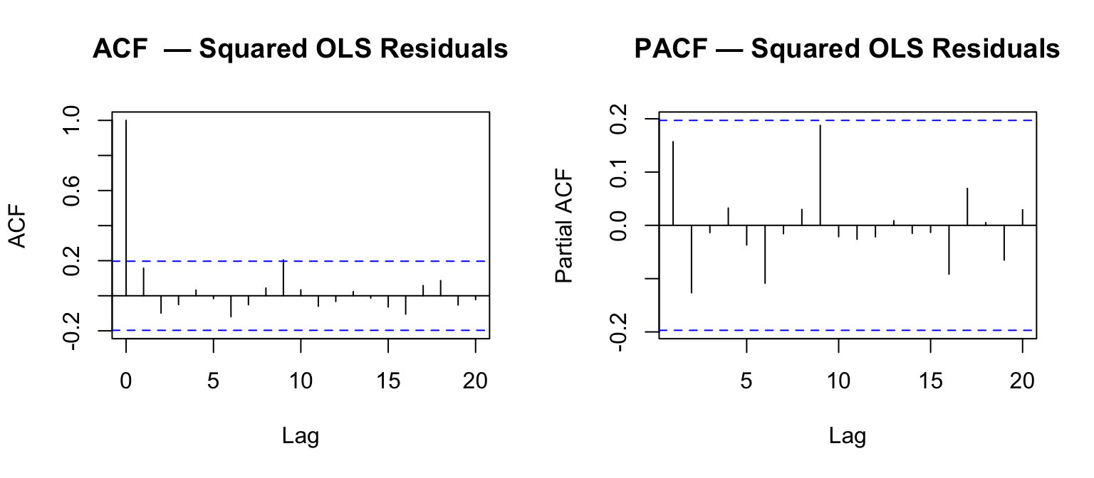
Autocorrelation in the squared OLS residuals signals ARCH effects.

# Align residuals into df by row index
df$resid_ols <- NA
df$resid_ols[as.integer(rownames(model.frame(reg_ecm)))] <- residuals(reg_ecm)
df$resid_ols_sq <- df$resid_ols^2

resid_sq_clean <- na.omit(df$resid_ols_sq)
par(mfrow = c(1, 2))
acf( resid_sq_clean, lag.max = 20, main = "ACF  — Squared OLS Residuals")
pacf(resid_sq_clean, lag.max = 20, main = "PACF — Squared OLS Residuals")

par(mfrow = c(1, 1))
predict resid_ols, res     /* 3 missing values generated */
gen resid_ols_sq = resid_ols * resid_ols
corrgram resid_ols_sq
* AC at lag 1 = 0.157, lag 9 = 0.205; no strong ARCH signal but proceed

8. ARCH(1) Model

We account for conditional heteroskedasticity. Iraq casualties (logged, lagged one period) enter the variance equation.

Note

Stata vs R — variance equation parameterisation

Stata’s het() option uses a multiplicative log-linear specification:

\[\sigma^2_t = \exp(\gamma_0 + \gamma_1 \cdot \text{L.casl})\,(1 + \alpha_1\,\varepsilon^2_{t-1})\]

Stata estimates: γ₀ = 2.509, γ₁ = −0.310, α₁ = 0.398.

rugarch’s external.regressors in the variance model uses an additive specification:

\[\sigma^2_t = \omega + \alpha_1\,\varepsilon^2_{t-1} + \eta\,\text{L.casl}\]

Because the true generating model is multiplicative, the additive form cannot represent it well: rugarch estimates vxreg1 (η) ≈ 0, absorbing the casualty effect into omega. The ARCH coefficient (α₁ = 0.380 vs Stata’s 0.398) and mean-equation slopes are nonetheless close.

Mean equation comparison (Stata → R):

Term Stata R (rugarch)
Intercept 5.248 5.045
labecmand 0.271 0.326
L.app −0.160 −0.146
L.labecman 0.135 0.110
v911d 9.677 9.807
petrold −6.377 −5.698
L2D.casl −3.058 −2.688
ARCH α₁ 0.398 0.380

8.1 Fit the Model

# Drop rows with any NA across required columns
arch_vars <- c("month", "dapp", "dlabecman", "L_app", "L_labecman",
               "v911d", "petrold", "L2Dcasl", "L_casl")
arch_df   <- na.omit(df[, arch_vars])

y_arch    <- arch_df$dapp
mean_xreg <- as.matrix(arch_df[, c("dlabecman", "L_app", "L_labecman",
                                    "v911d", "petrold", "L2Dcasl")])
var_xreg  <- as.matrix(arch_df[, "L_casl", drop = FALSE])

spec_arch <- ugarchspec(
  variance.model = list(
    model               = "sGARCH",
    garchOrder          = c(1, 0),   # ARCH(1): one alpha, no beta
    external.regressors = var_xreg   # additive approximation to het(L.casl)
  ),
  mean.model = list(
    armaOrder           = c(0, 0),
    include.mean        = TRUE,
    external.regressors = mean_xreg
  ),
  distribution.model = "norm"
)

fit_arch <- ugarchfit(spec = spec_arch, data = y_arch)
Warning in .sgarchfit(spec = spec, data = data, out.sample = out.sample, : 
ugarchfit-->waring: using less than 100 data
 points for estimation
show(fit_arch)

*---------------------------------*
*          GARCH Model Fit        *
*---------------------------------*

Conditional Variance Dynamics   
-----------------------------------
GARCH Model : sGARCH(1,0)
Mean Model  : ARFIMA(0,0,0)
Distribution    : norm 

Optimal Parameters
------------------------------------
        Estimate  Std. Error  t value Pr(>|t|)
mu       5.04534    1.677470   3.0077 0.002632
mxreg1   0.32596    0.103955   3.1356 0.001715
mxreg2  -0.14625    0.053338  -2.7420 0.006107
mxreg3   0.11005    0.071776   1.5333 0.125204
mxreg4   9.80731    1.964128   4.9932 0.000001
mxreg5  -5.69816    2.099639  -2.7139 0.006650
mxreg6  -2.68849    1.174041  -2.2899 0.022024
omega    9.22671    2.200012   4.1939 0.000027
alpha1   0.38039    0.211936   1.7948 0.072679
vxreg1   0.00000    1.614627   0.0000 1.000000

Robust Standard Errors:
        Estimate  Std. Error  t value Pr(>|t|)
mu       5.04534    1.228585  4.10663 0.000040
mxreg1   0.32596    0.132321  2.46340 0.013763
mxreg2  -0.14625    0.046390 -3.15264 0.001618
mxreg3   0.11005    0.073907  1.48908 0.136465
mxreg4   9.80731    1.568366  6.25320 0.000000
mxreg5  -5.69816    1.526430 -3.73300 0.000189
mxreg6  -2.68849    2.010394 -1.33730 0.181126
omega    9.22671    2.920220  3.15959 0.001580
alpha1   0.38039    0.452385  0.84086 0.400427
vxreg1   0.00000    4.380768  0.00000 1.000000

LogLikelihood : -267.2461 

Information Criteria
------------------------------------
                   
Akaike       5.6009
Bayes        5.8631
Shibata      5.5829
Hannan-Quinn 5.7070

Weighted Ljung-Box Test on Standardized Residuals
------------------------------------
                        statistic p-value
Lag[1]                     0.4069  0.5235
Lag[2*(p+q)+(p+q)-1][2]    2.3843  0.2063
Lag[4*(p+q)+(p+q)-1][5]    3.6709  0.2980
d.o.f=0
H0 : No serial correlation

Weighted Ljung-Box Test on Standardized Squared Residuals
------------------------------------
                        statistic p-value
Lag[1]                    0.02791  0.8673
Lag[2*(p+q)+(p+q)-1][2]   0.22850  0.8369
Lag[4*(p+q)+(p+q)-1][5]   0.44433  0.9659
d.o.f=1

Weighted ARCH LM Tests
------------------------------------
            Statistic Shape Scale P-Value
ARCH Lag[2]    0.3853 0.500 2.000  0.5348
ARCH Lag[4]    0.4909 1.397 1.611  0.8711
ARCH Lag[6]    1.1119 2.222 1.500  0.8738

Nyblom stability test
------------------------------------
Joint Statistic:  2.6979
Individual Statistics:               
mu     0.165399
mxreg1 0.195088
mxreg2 0.182509
mxreg3 0.147135
mxreg4 0.005973
mxreg5 0.005061
mxreg6 0.008980
omega  0.165220
alpha1 0.031573
vxreg1 1.173247

Asymptotic Critical Values (10% 5% 1%)
Joint Statistic:         2.29 2.54 3.05
Individual Statistic:    0.35 0.47 0.75

Sign Bias Test
------------------------------------
                   t-value   prob sig
Sign Bias           0.1834 0.8549    
Negative Sign Bias  0.3626 0.7177    
Positive Sign Bias  0.2948 0.7688    
Joint Effect        0.9558 0.8120    


Adjusted Pearson Goodness-of-Fit Test:
------------------------------------
  group statistic p-value(g-1)
1    20     11.91       0.8895
2    30     27.36       0.5521
3    40     36.35       0.5912
4    50     58.07       0.1758


Elapsed time : 0.176755 
* appd and labecmand are pre-differenced variables already in the dataset.
* het(L.casl) uses a multiplicative log-linear variance model (see note above).
arch appd labecmand L.app L.labecman v911d petrold L2D.casl, ///
     het(L.casl) arch(1)
* Log L = -263.06; N = 99; sample 1997m10 to 2005m12
* HET: L.casl = -0.310 (p=0.003), _cons = 2.509 (p<0.001)
* ARCH L1 = 0.398 (p=0.032)

8.2 Residual Diagnostics

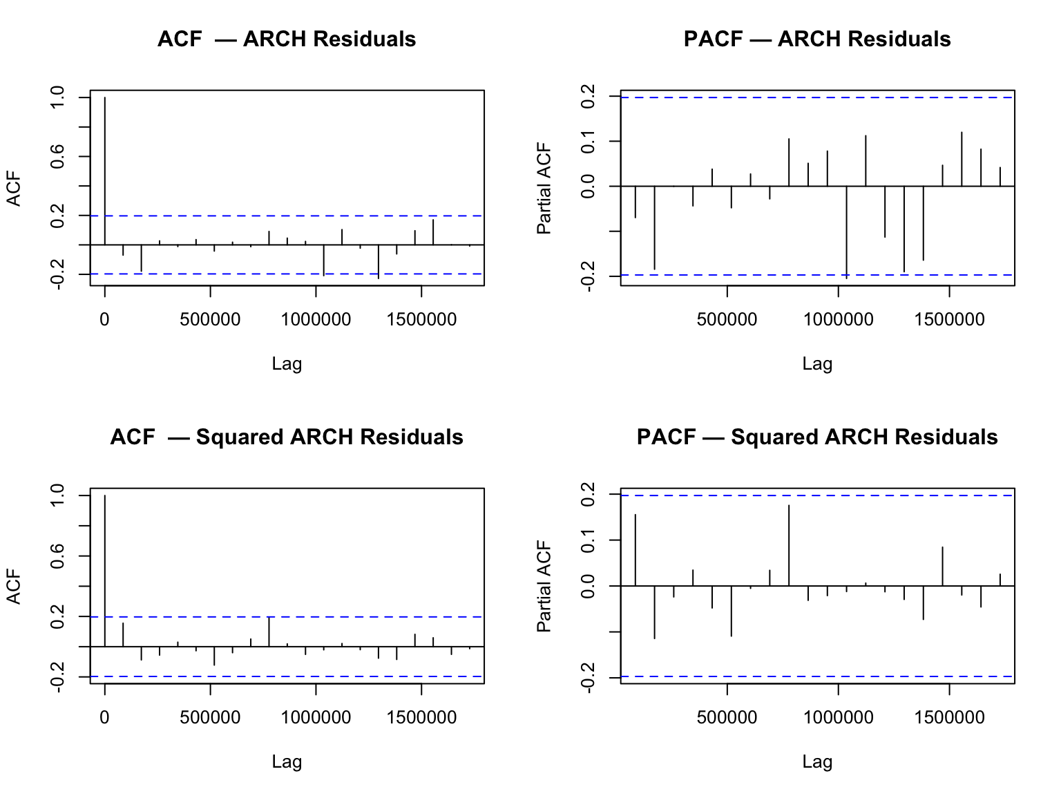
If the model is well-specified, neither the residuals nor their squares should show significant autocorrelation.

resid_arch    <- residuals(fit_arch)
resid_arch_sq <- resid_arch^2

par(mfrow = c(2, 2))
acf( resid_arch,    lag.max = 20, main = "ACF  — ARCH Residuals")
pacf(resid_arch,    lag.max = 20, main = "PACF — ARCH Residuals")
acf( resid_arch_sq, lag.max = 20, main = "ACF  — Squared ARCH Residuals")
pacf(resid_arch_sq, lag.max = 20, main = "PACF — Squared ARCH Residuals")

par(mfrow = c(1, 1))
predict resid, res     /* 3 missing values generated */
corrgram resid         /* no significant autocorrelation */

gen resid_sq = resid * resid
corrgram resid_sq      /* no significant autocorrelation */

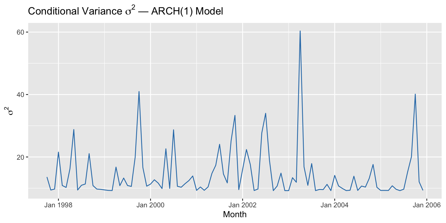
8.3 Conditional Variance

sigma2    <- sigma(fit_arch)^2   # sigma() returns std dev; square for variance
sigma2_df <- data.frame(
  month  = arch_df$month,
  sigma2 = as.numeric(sigma2)
)

ggplot(sigma2_df, aes(x = month, y = sigma2)) +
  geom_line(colour = "#2c7bb6") +
  labs(
    title = expression("Conditional Variance " * sigma^2 * " — ARCH(1) Model"),
    x = "Month", y = expression(sigma^2)
  )

predict sigma2, variance   /* 1 missing value generated */
graph twoway line sigma2 month

9. Digression: Random Walks

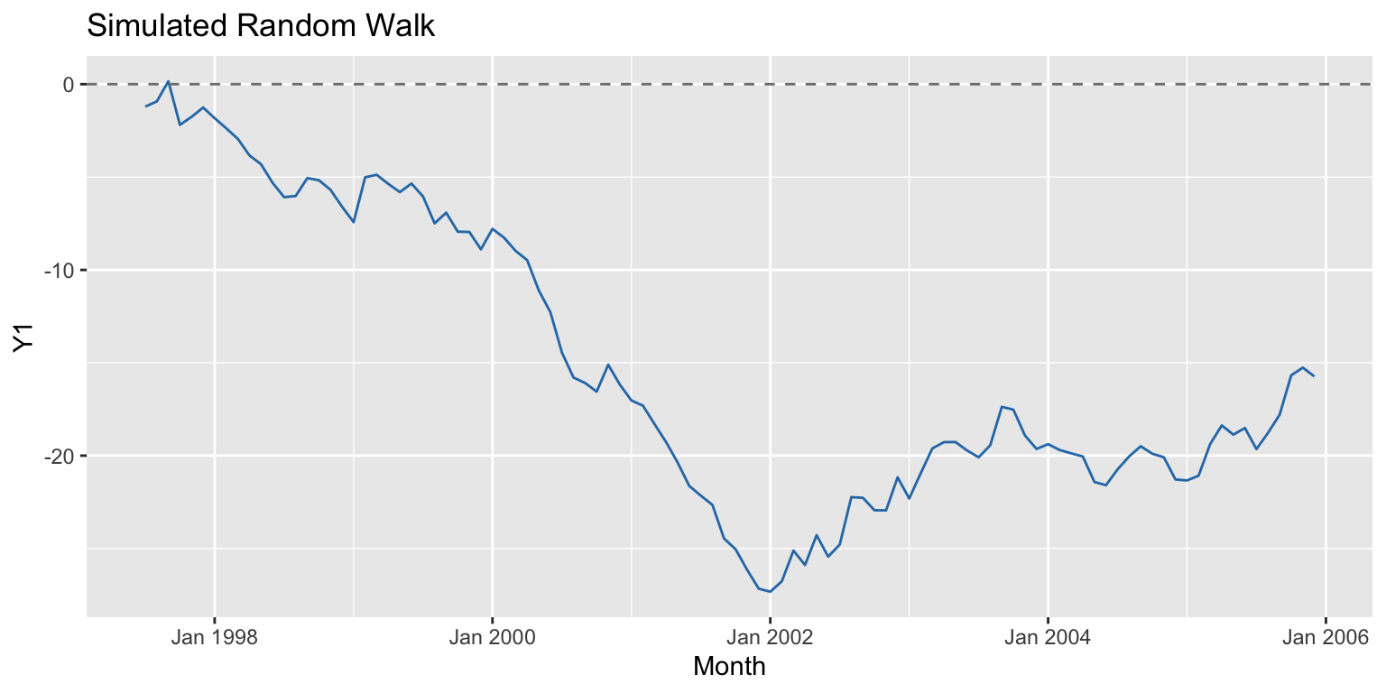
Random walks are non-stationary with variance growing over time. We simulate one and confirm the ARCH model detects time-varying variance.

Note

R and Stata use different random number generators. Even with the same seed (1234), rnorm() and drawnorm produce different sequences, so the simulated paths diverge. Consequently, the ARCH model results (mean, omega, alpha) will also differ between platforms — this is expected, not an error.

9.1 Simulate and Plot

set.seed(1234)
r1 <- rnorm(n)       # one N(0,1) draw per observation
Y1 <- cumsum(r1)     # cumsum() = Stata's running sum()

rw_df <- data.frame(month = df$month, Y1 = Y1)
ggplot(rw_df, aes(x = month, y = Y1)) +
  geom_line(colour = "#2c7bb6") +
  geom_hline(yintercept = 0, linetype = "dashed", colour = "grey50") +
  labs(title = "Simulated Random Walk", x = "Month", y = "Y1")

set seed 1234
drawnorm r1               /* different RNG from R's rnorm() */
generate Y1 = sum(r1)     /* sum() in Stata is a running/cumulative sum */
twoway line Y1 month, yline(0)
* Stata path mean ≈ 4.3; R path mean ≈ -19.5 — different due to RNG

9.2 ARCH(1) on the Random Walk

rw_spec <- ugarchspec(
  variance.model     = list(model = "sGARCH", garchOrder = c(1, 0)),
  mean.model         = list(armaOrder = c(0, 0), include.mean = TRUE),
  distribution.model = "norm"
)
rw_fit <- ugarchfit(spec = rw_spec, data = Y1)
show(rw_fit)

*---------------------------------*
*          GARCH Model Fit        *
*---------------------------------*

Conditional Variance Dynamics   
-----------------------------------
GARCH Model : sGARCH(1,0)
Mean Model  : ARFIMA(0,0,0)
Distribution    : norm 

Optimal Parameters
------------------------------------
        Estimate  Std. Error  t value Pr(>|t|)
mu     -19.49807     0.26690 -73.0548  0.00000
omega    0.71399     0.25562   2.7931  0.00522
alpha1   0.93836     0.16158   5.8073  0.00000

Robust Standard Errors:
        Estimate  Std. Error  t value Pr(>|t|)
mu     -19.49807    0.519715 -37.5168 0.000000
omega    0.71399    0.201891   3.5365 0.000405
alpha1   0.93836    0.069567  13.4885 0.000000

LogLikelihood : -288.5026 

Information Criteria
------------------------------------
                   
Akaike       5.7157
Bayes        5.7929
Shibata      5.7141
Hannan-Quinn 5.7470

Weighted Ljung-Box Test on Standardized Residuals
------------------------------------
                        statistic p-value
Lag[1]                      70.82       0
Lag[2*(p+q)+(p+q)-1][2]     97.32       0
Lag[4*(p+q)+(p+q)-1][5]    158.92       0
d.o.f=0
H0 : No serial correlation

Weighted Ljung-Box Test on Standardized Squared Residuals
------------------------------------
                        statistic p-value
Lag[1]                     0.6161  0.4325
Lag[2*(p+q)+(p+q)-1][2]    0.8337  0.5554
Lag[4*(p+q)+(p+q)-1][5]    3.0392  0.3999
d.o.f=1

Weighted ARCH LM Tests
------------------------------------
            Statistic Shape Scale P-Value
ARCH Lag[2]    0.4186 0.500 2.000  0.5176
ARCH Lag[4]    2.2689 1.397 1.611  0.3840
ARCH Lag[6]    3.9363 2.222 1.500  0.3165

Nyblom stability test
------------------------------------
Joint Statistic:  0.4416
Individual Statistics:              
mu     0.26288
omega  0.01650
alpha1 0.07609

Asymptotic Critical Values (10% 5% 1%)
Joint Statistic:         0.846 1.01 1.35
Individual Statistic:    0.35 0.47 0.75

Sign Bias Test
------------------------------------
                   t-value   prob sig
Sign Bias           0.3849 0.7012    
Negative Sign Bias  0.3680 0.7137    
Positive Sign Bias  0.1269 0.8993    
Joint Effect        0.1802 0.9807    


Adjusted Pearson Goodness-of-Fit Test:
------------------------------------
  group statistic p-value(g-1)
1    20     174.1    4.512e-27
2    30     203.3    4.454e-28
3    40     240.0    9.679e-31
4    50     233.3    8.102e-26


Elapsed time : 0.02026701 
arch Y1, arch(1)
* _cons = 4.264, ARCH L1 = 1.001 (≈1: variance growing at rate of random walk)
* omega = 0.517
* R results differ due to different simulated path (see RNG note above)

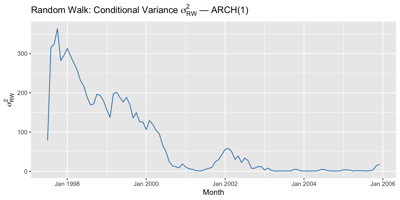
9.3 Conditional Variance of the Random Walk

sigma1_rw   <- sigma(rw_fit)^2
sigma_rw_df <- data.frame(
  month     = df$month[seq_along(sigma1_rw)],
  sigma1_rw = as.numeric(sigma1_rw)
)

ggplot(sigma_rw_df, aes(x = month, y = sigma1_rw)) +
  geom_line(colour = "#2c7bb6") +
  labs(
    title = expression("Random Walk: Conditional Variance " *
                       sigma[RW]^2 * " — ARCH(1)"),
    x = "Month", y = expression(sigma[RW]^2)
  )

predict sigma1_rw, variance
graph twoway line sigma1_rw month
* Both R and Stata show increasing variance — the key qualitative result