Day 7: Missing Data

Slides

• A reveal presentation for Day 6
• A reveal presentation on CFR’s
• A reveal presentation on Multiple Imputation

Cross-sectional time series (TSCS) data — also called panel or longitudinal data — pose particular challenges for multiple imputation. Standard imputation methods treat observations as exchangeable, discarding two structural features that TSCS data possess in abundance:

1. Temporal autocorrelation: an observation for unit \(i\) at time \(t\) is predictable from observations for the same unit at \(t \pm 1, t \pm 2, \ldots\)
2. Unit-specific trajectories: each cross-sectional unit follows its own trend over time, so a pooled time polynomial is too restrictive.

Honaker and King (2010, AJPS 54:561–581) adapt the EM algorithm to exploit both features. Their software — Amelia II — augments every imputation equation with polynomial functions of time interacted with unit indicators, letting the model borrow information from temporal neighbours within each unit. This recovers much of the information discarded by listwise deletion, which in TSCS settings tends to cluster in time and across units (making the MCAR assumption implausible).

Why This Matters for Human Rights Research

The Poe–Tate–Keith (PTK) model of state repression is a canonical application of TSCS analysis in comparative politics. Its central predictor — democracy — is systematically missing in ways that are almost certainly non-random: authoritarian regimes are more likely both to repress citizens and to lack reliable democracy scores. Standard listwise deletion therefore discards precisely those observations most likely to illuminate the democracy–repression relationship, biasing coefficients toward zero (or even reversing signs). Because democracy scores for a country in year \(t\) are strongly predicted by scores in years \(t-1\) and \(t+1\), the MAR assumption is far more defensible than it first appears — the temporal neighbours act as observed proxies for the unobserved value.

The Missing-Data Taxonomy

Mechanism	Condition	Consequence for estimators
MCAR	\(P(\mathbf{M} \mid \mathbf{Y}) = P(\mathbf{M})\)	Listwise deletion is unbiased but inefficient
MAR	\(P(\mathbf{M} \mid \mathbf{Y}) = P(\mathbf{M} \mid \mathbf{Y}_\text{obs})\)	MI is consistent and efficient
MNAR	Depends on unobserved values	No off-the-shelf solution; sensitivity analysis required

Honaker and King argue that the MAR assumption is more defensible in TSCS data than it first appears: temporal neighbours of a missing value act as proxies for what was not observed, so the probability of missingness depends primarily on observed quantities.

Rubin’s Combining Rules

Given \(M\) imputed datasets, estimate the quantity of interest \(Q\) in each dataset, obtaining \(\hat{Q}_m\) with estimated variance \(\hat{U}_m\). Rubin (1987) shows valid frequentist inference follows from:

\[\bar{Q} = \frac{1}{M}\sum_{m=1}^{M}\hat{Q}_m\]

\[\bar{U} = \frac{1}{M}\sum_{m=1}^{M}\hat{U}_m \qquad \text{(within-imputation variance)}\]

\[B = \frac{1}{M-1}\sum_{m=1}^{M}(\hat{Q}_m - \bar{Q})^2 \qquad \text{(between-imputation variance)}\]

\[T = \bar{U} + \left(1 + \frac{1}{M}\right)B \qquad \text{(total variance)}\]

The fraction of missing information (FMI) summarises how much the missing data inflate posterior uncertainty:

\[\hat{\gamma} = \frac{(1 + 1/M)\,B}{T}\]

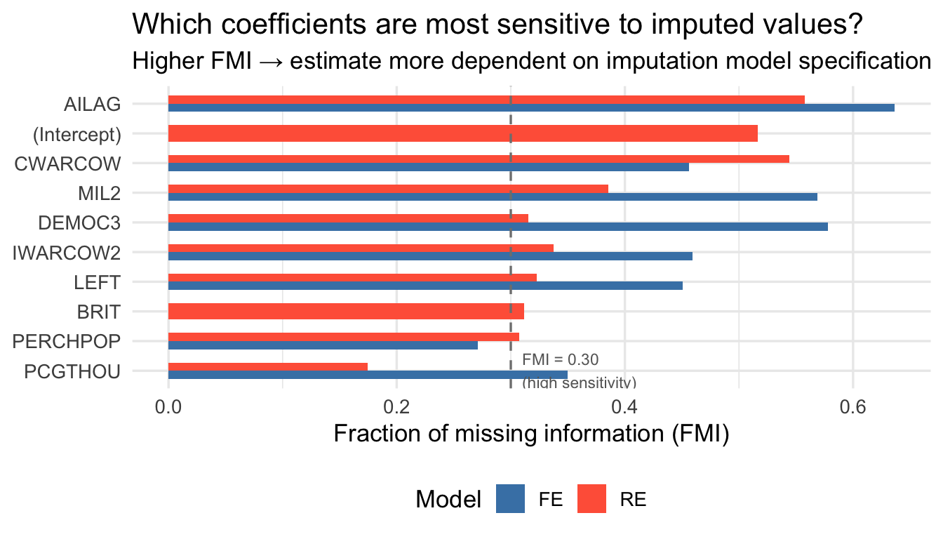
A large FMI on the DEMOC3 coefficient would confirm that our inference about the democracy–repression relationship is sensitive to imputation model choices — exactly what we would expect given the non-random pattern of missingness.

The Barnard–Rubin (1999) small-sample degrees of freedom are:

\[\nu = (M-1)\!\left[1 + \frac{M\bar{U}}{(M+1)B}\right]^{2}\]

These are what mi estimate in Stata and mi.meld() in R implement.

---

Data: Poe, Tate & Keith (1999)

We use the ISQ99-Essex dataset from Poe, Tate, and Keith’s (1999) study of the determinants of state repression, published in the International Studies Quarterly. The dataset covers a broad cross-national panel and pairs two dependent variables — Amnesty International (AI) and State Department (SD) human rights scores — with a standard set of structural predictors. The central theoretical claim is that democracy substantially reduces physical integrity rights violations, holding constant war, economic development, population, regime type, and colonial history.

The dataset is available directly from GitHub as a Stata .dta file, which both R (haven) and Stata can read from the URL without local download.

Variable	Description	Scale
AINEW	Physical integrity rights score (Amnesty International)	Ordinal 1–5 (higher = more repression)
AILAG	Lagged AI score (year \(t-1\))	Ordinal 1–5
SDNEW	Physical integrity rights score (State Department)	Ordinal 1–5
SDLAG	Lagged SD score	Ordinal 1–5
POLRT	Political rights	Ordinal
DEMOC3	Democracy indicator (primary variable with missingness)	Continuous
PCGTHOU	GDP per capita (thousands USD)	Continuous
PERCHPCG	Annual percent change in per capita GDP	Continuous
PERCHPOP	Annual percent change in population	Continuous
LPOP	Log population	Continuous
CWARCOW	Civil war (Correlates of War)	Binary
IWARCOW2	Interstate war (Correlates of War)	Binary
MIL2	Military government	Binary
LEFT	Left-wing government	Binary
BRIT	British colonial heritage (time-invariant)	Binary
IDORIGIN	Country identifier	Panel ID
YEAR	Year	Time ID

Note

BRIT is a time-invariant country characteristic. It will be absorbed by unit fixed effects in the FE estimator and will drop out, but it remains a useful predictor in the imputation model and the random-effects specification.

R

# Load directly from the GitHub URL — no local copy needed
ISQ99_Essex <- read_dta(
  "https://github.com/robertwwalker/Essex-Data/raw/main/ISQ99-Essex.dta"
)

# haven returns labelled vectors; strip labels to plain numerics/characters
# so that Amelia and plm receive clean data frames
ISQ99_Essex <- zap_labels(ISQ99_Essex)

glimpse(ISQ99_Essex)

Rows: 3,222
Columns: 21
$ IDORIGIN <dbl> 2, 2, 2, 2, 2, 2, 2, 2, 2, 2, 2, 2, 2, 2, 2, 2, 2, 2, 20, 20,…
$ YEAR     <dbl> 1976, 1977, 1978, 1979, 1980, 1981, 1982, 1983, 1984, 1985, 1…
$ AI       <dbl> 1, 1, 1, 1, 1, 1, 1, 1, 1, 1, 1, 2, 1, 1, 1, 2, 2, 1, 1, NA, …
$ SD       <dbl> NA, 1, NA, NA, NA, NA, NA, NA, NA, NA, NA, NA, NA, NA, NA, NA…
$ POLRT    <dbl> 7, 7, 7, 7, 7, 7, 7, 7, 7, 7, 7, 7, 7, 7, 7, 7, 7, 7, 7, 7, 7…
$ MIL2     <dbl> 0, 0, 0, 0, 0, 0, 0, 0, 0, 0, 0, 0, 0, 0, 0, 0, 0, 0, 0, 0, 0…
$ LEFT     <dbl> 0, 0, 0, 0, 0, 0, 0, 0, 0, 0, 0, 0, 0, 0, 0, 0, 0, 0, 0, 0, 0…
$ BRIT     <dbl> 1, 1, 1, 1, 1, 1, 1, 1, 1, 1, 1, 1, 1, 1, 1, 1, 1, 1, 1, 1, 1…
$ PCGNP    <dbl> 8190, 9070, 10140, 11200, 12040, 13370, 13710, 14600, 16050, …
$ AINEW    <dbl> 1, 1, 1, 1, 1, 1, 1, 1, 1, 1, 1, 2, 1, 1, 1, 2, 2, 1, 1, 1, 1…
$ SDNEW    <dbl> 1, 1, 1, 1, 1, 1, 1, 1, 1, 1, 1, 2, 1, 1, 1, 2, 2, 1, 1, 1, 1…
$ IDGURR   <dbl> 2, 2, 2, 2, 2, 2, 2, 2, 2, 2, 2, 2, 2, 2, 2, 2, 2, 2, 20, 20,…
$ AILAG    <dbl> NA, 1, 1, 1, 1, 1, 1, 1, 1, 1, 1, 1, 2, 1, 1, 1, 2, 2, NA, 1,…
$ SDLAG    <dbl> NA, 1, 1, 1, 1, 1, 1, 1, 1, 1, 1, 1, 2, 1, 1, 1, 2, 2, NA, 1,…
$ PERCHPCG <dbl> NA, 10.74, 11.80, 10.45, 7.50, 11.05, 2.54, 6.49, 9.93, 5.36,…
$ PERCHPOP <dbl> NA, 1.01, 1.07, 1.11, 1.20, 1.05, 1.04, 0.98, 0.94, 0.96, 0.9…
$ LPOP     <dbl> 19.20, 19.21, 19.22, 19.23, 19.24, 19.25, 19.26, 19.27, 19.28…
$ PCGTHOU  <dbl> 8.19, 9.07, 10.14, 11.20, 12.04, 13.37, 13.71, 14.60, 16.05, …
$ DEMOC3   <dbl> 10, 10, 10, 10, 10, 10, 10, 10, 10, 10, 10, 10, 10, 10, 10, 1…
$ CWARCOW  <dbl> 0, 0, 0, 0, 0, 0, 0, 0, 0, 0, 0, 0, 0, 0, 0, 0, 0, 0, 0, 0, 0…
$ IWARCOW2 <dbl> 0, 0, 0, 0, 0, 0, 0, 0, 0, 0, 0, 0, 0, 0, 1, 1, 1, 1, 0, 0, 0…

# Declare a pdata.frame so that plm functions (pvar, is.pbalanced, etc.) work
ISQ99p <- pdata.frame(ISQ99_Essex, index = c("IDORIGIN", "YEAR"))

# Is the panel balanced?
is.pbalanced(ISQ99p)

[1] TRUE

# Which variables are time-invariant (pure cross-section) or
# individual-invariant (pure time series)?
# pvar() flags variables with zero within-unit variation (tv = FALSE)
# or zero between-unit variation (ti = FALSE).
pvar(ISQ99p)

no time variation:       IDORIGIN BRIT IDGURR AILAG SDLAG PERCHPCG PERCHPOP 
no individual variation: YEAR AI SD POLRT MIL2 LEFT BRIT PCGNP AINEW SDNEW AILAG SDLAG PERCHPCG PERCHPOP LPOP PCGTHOU DEMOC3 CWARCOW IWARCOW2 
all NA in time dimension for at least one individual:  AI SD POLRT MIL2 LEFT BRIT PCGNP AINEW SDNEW AILAG SDLAG PERCHPCG PERCHPOP LPOP PCGTHOU DEMOC3 CWARCOW IWARCOW2 
all NA in ind. dimension for at least one time period: AI SD POLRT MIL2 LEFT BRIT PCGNP AINEW SDNEW AILAG SDLAG PERCHPCG PERCHPOP LPOP PCGTHOU DEMOC3 CWARCOW IWARCOW2 

Stata

* Load directly from GitHub — Stata accepts https:// URLs for use
use "https://github.com/robertwwalker/Essex-Data/raw/main/ISQ99-Essex.dta", clear

describe
label list    // inspect value labels if any

* Declare as panel data
xtset IDORIGIN YEAR

* Check panel balance
xtdescribe

* Time-invariant variables (BRIT should appear constant within units)
bysort IDORIGIN: egen sd_BRIT = sd(BRIT)
tab sd_BRIT    // should be 0 for all — confirms BRIT is time-invariant
drop sd_BRIT

---

Missingness Patterns

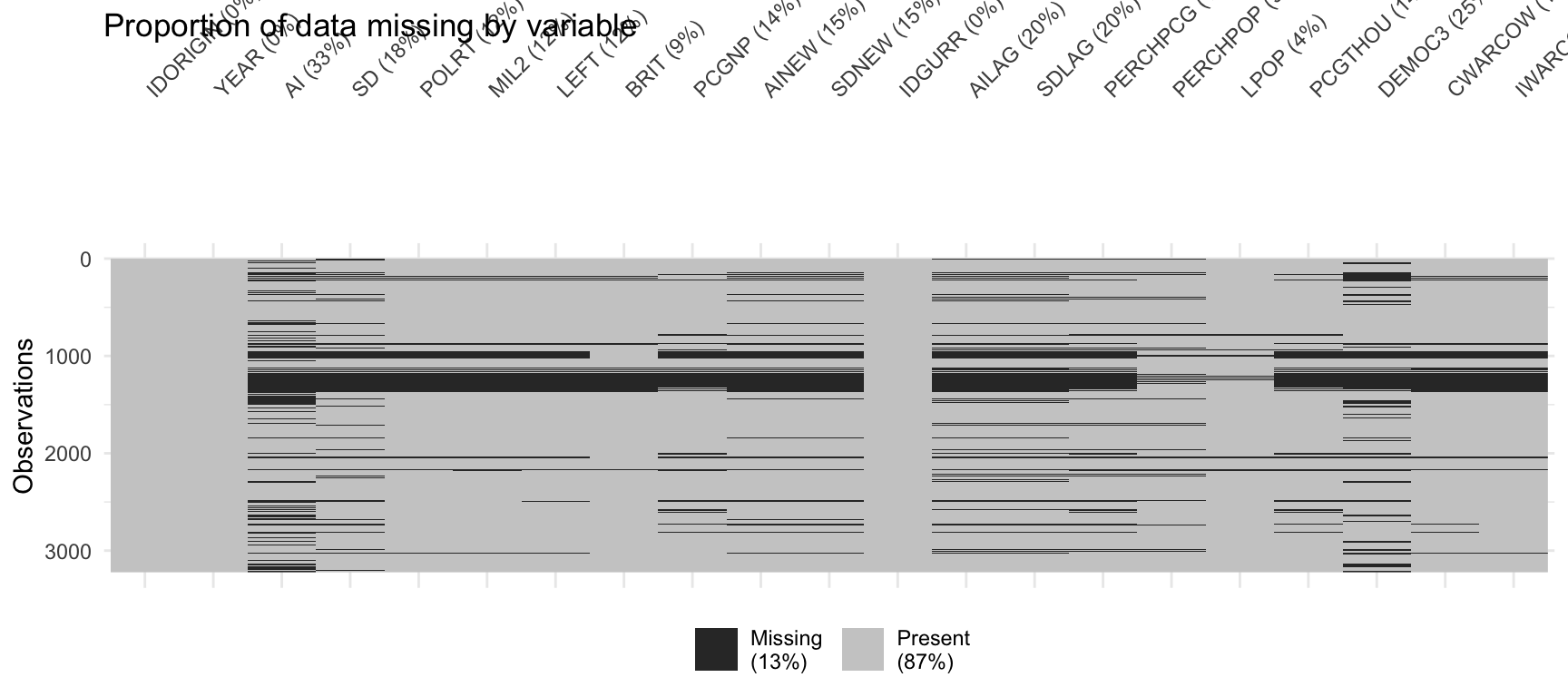
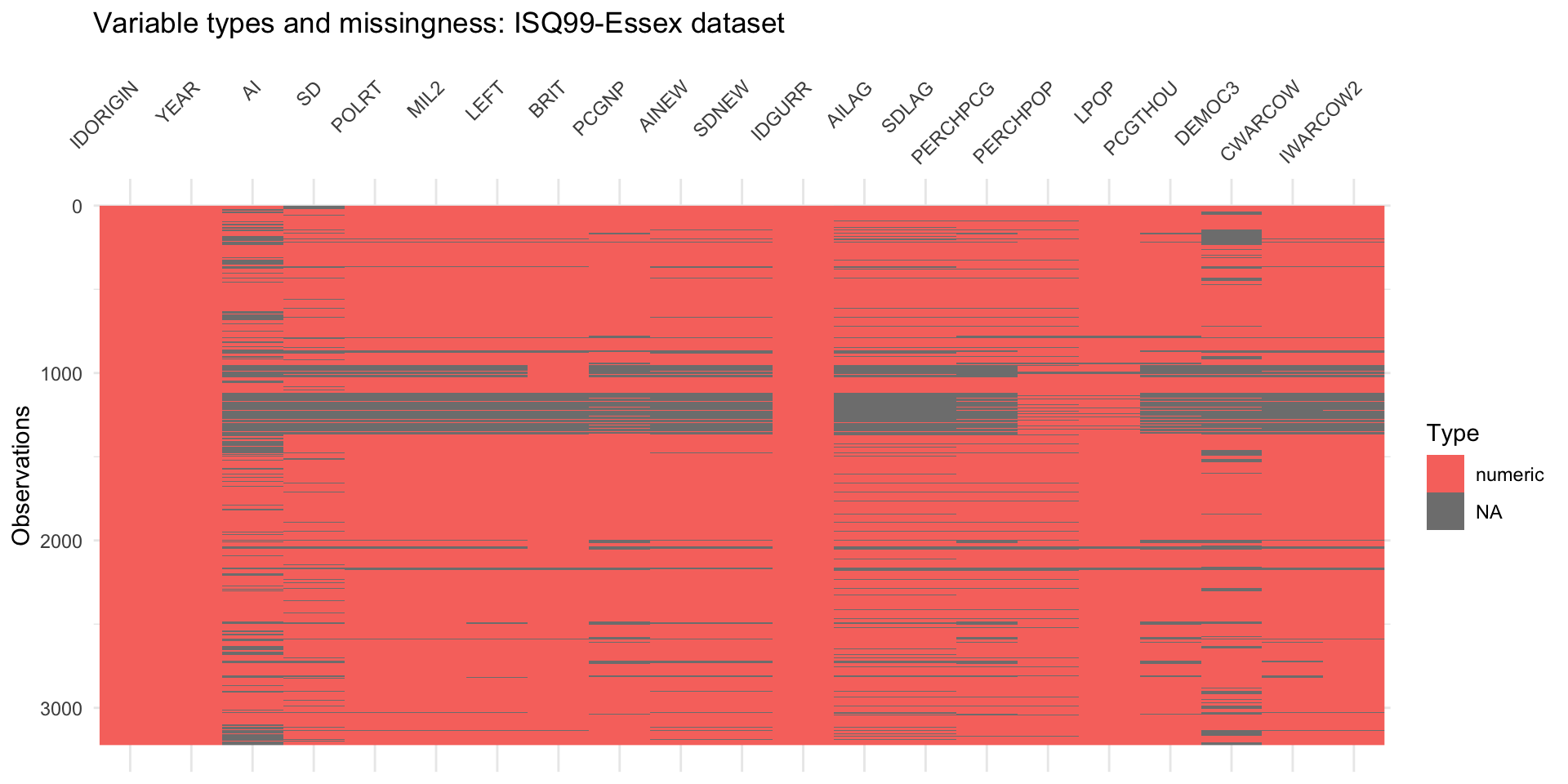
Before imputing, it is essential to understand where data are missing and whether the pattern is consistent with the MAR assumption. For the PTK model, the key concern is that DEMOC3 is missing disproportionately for countries that are also authoritarian repressors — a pattern that would make MCAR untenable.

Aggregate patterns

R

# Overview of all variable types and missingness simultaneously
vis_dat(ISQ99_Essex) +
  labs(title = "Variable types and missingness: ISQ99-Essex dataset") +
  theme(axis.text.x = element_text(angle = 45, hjust = 1))

# Proportion missing per variable, sorted
vis_miss(ISQ99_Essex) +
  labs(title = "Proportion of data missing by variable")

miss_var_summary(ISQ99_Essex) |>
  filter(n_miss > 0) |>
  gt() |>
  tab_header(title = "Missing data summary — ISQ99-Essex") |>
  fmt_number(columns = pct_miss, decimals = 1) |>
  cols_label(variable = "Variable", n_miss = "N missing", pct_miss = "% missing") |>
  tab_footnote(
    footnote = "DEMOC3 is the key democracy predictor; its missingness drives most of the MI rationale.",
    locations = cells_body(columns = variable, rows = variable == "DEMOC3")
  )

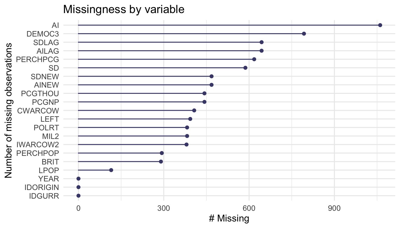
Missing data summary — ISQ99-Essex
Variable	N missing	% missing
AI	1061	32.9
DEMOC31	793	24.6
AILAG	644	20.0
SDLAG	644	20.0
PERCHPCG	618	19.2
SD	587	18.2
AINEW	468	14.5
SDNEW	468	14.5
PCGNP	443	13.7
PCGTHOU	443	13.7
CWARCOW	407	12.6
LEFT	393	12.2
POLRT	382	11.9
MIL2	382	11.9
IWARCOW2	380	11.8
PERCHPOP	293	9.09
BRIT	290	9.00
LPOP	115	3.57
1 DEMOC3 is the key democracy predictor; its missingness drives most of the MI rationale.

# Univariate missingness — which variables lose the most observations?
gg_miss_var(ISQ99_Essex) +
  labs(title = "Missingness by variable",
       x = "Number of missing observations") +
  theme_minimal(base_size = 12)

Stata

* Summary of missing values per variable
misstable summarize DEMOC3 PCGTHOU POLRT AINEW AILAG

* Pattern of co-missingness (which combinations occur together?)
misstable patterns DEMOC3 PCGTHOU POLRT, frequency

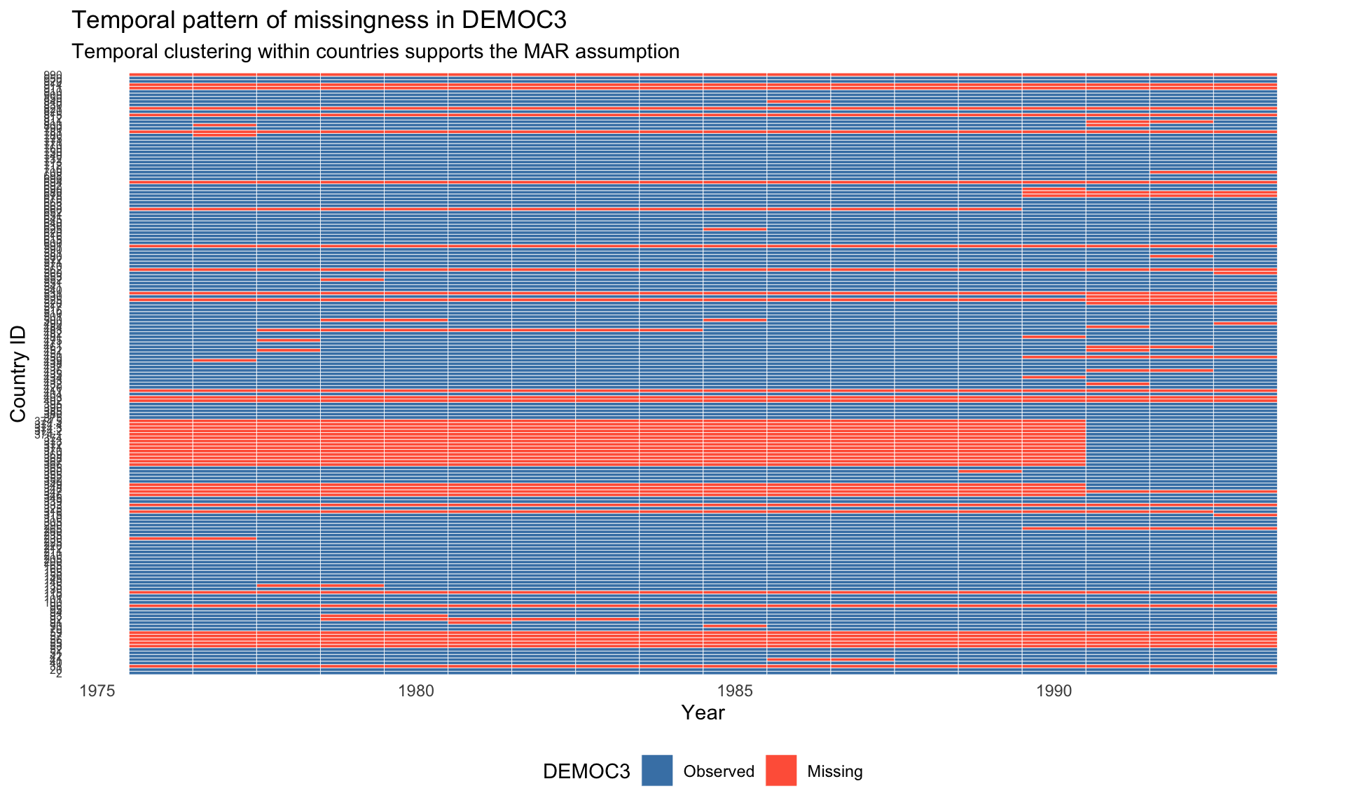
Temporal pattern of missingness in DEMOC3

The spatial and temporal clustering of missing democracy scores is the diagnostic most relevant to the H-K argument. If missingness is randomly scattered over time and countries, MCAR might be plausible. If it clusters — in certain years or certain countries — the TSCS imputation model’s ability to borrow from temporal neighbours becomes crucial.

R

# Tile plot: observed (blue) vs missing (red) DEMOC3 for each country-year
ISQ99_Essex |>
  mutate(democ_missing = is.na(DEMOC3)) |>
  ggplot(aes(x = YEAR, y = factor(IDORIGIN), fill = democ_missing)) +
  geom_tile(colour = "white", linewidth = 0.15) +
  scale_fill_manual(
    values = c("FALSE" = "steelblue", "TRUE" = "tomato"),
    labels = c("Observed", "Missing"),
    name   = "DEMOC3"
  ) +
  labs(
    title    = "Temporal pattern of missingness in DEMOC3",
    subtitle = "Temporal clustering within countries supports the MAR assumption",
    x = "Year", y = "Country ID"
  ) +
  theme_minimal(base_size = 11) +
  theme(
    legend.position  = "bottom",
    axis.text.y      = element_text(size = 6),
    panel.grid.major = element_blank()
  )

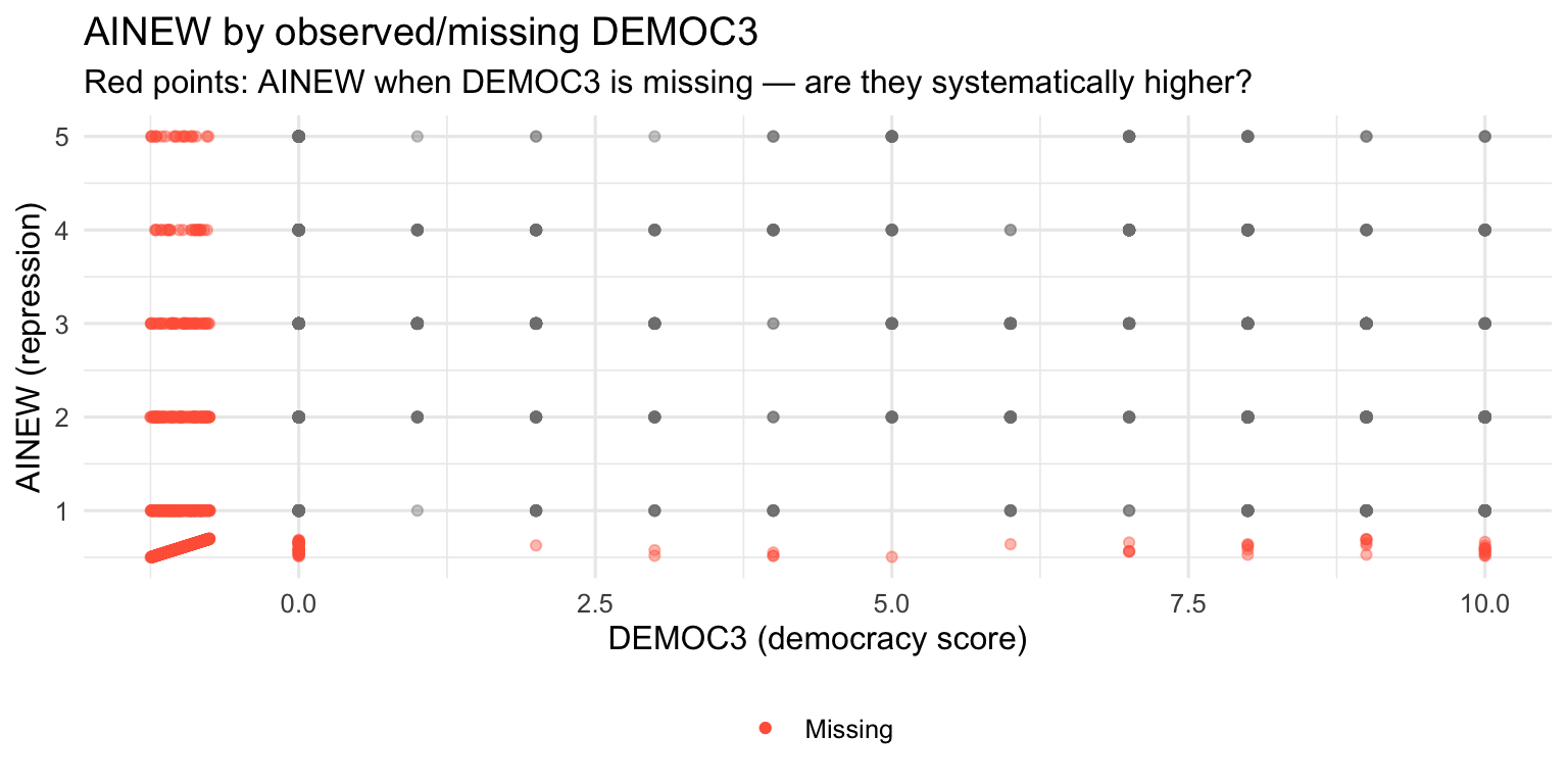
# Bivariate: how does AINEW vary with observed vs missing DEMOC3?
# geom_miss_point() colours observed points by the other variable's missingness.
# If AINEW distributions differ between observed and missing DEMOC3,
# that confirms missingness is NOT MCAR.
p_miss <- ggplot(ISQ99_Essex,
                 aes(x = DEMOC3, y = AINEW)) +
  geom_miss_point(alpha = 0.4) +
  scale_colour_manual(
    values = c("!Missing" = "steelblue", "Missing"  = "tomato"),
    name   = NULL
  ) +
  labs(
    title    = "AINEW by observed/missing DEMOC3",
    subtitle = "Red points: AINEW when DEMOC3 is missing — are they systematically higher?",
    x = "DEMOC3 (democracy score)", y = "AINEW (repression)"
  ) +
  theme_minimal(base_size = 12) +
  theme(legend.position = "bottom")

p_miss

Tip

If the red points (AINEW values when DEMOC3 is missing) cluster at higher values of AINEW, this is direct evidence that missingness in democracy data is related to the outcome — the most repressive countries are the ones with missing democracy scores. This pattern is exactly what makes MCAR implausible and MAR (with temporal borrowing) the right working assumption.

Stata

* Proportion of DEMOC3 missing by year
bysort YEAR: egen n_miss_D = total(missing(DEMOC3))
bysort YEAR: gen  n_obs    = _N
gen pct_miss_D = n_miss_D / n_obs * 100
label variable pct_miss_D "% DEMOC3 missing"

* Is the distribution of AINEW different when DEMOC3 is missing?
ttest AINEW, by(missing(DEMOC3))
* A significant difference = MCAR is implausible

* Visualise missingness pattern by year (tabplot from SSC)
* ssc install tabplot, replace
tabplot IDORIGIN YEAR if missing(DEMOC3), ///
    title("Country-years with missing DEMOC3") scheme(s2color)

---

Imputation with Amelia

Amelia fits an expectation-maximisation with importance sampling (EMis) model under the assumption of approximate multivariate normality. For TSCS data, Honaker and King (2010) recommend the following additional options, which we implement below.

Argument	Purpose
ts = "YEAR"	Identifies the time variable
cs = "IDORIGIN"	Identifies the cross-sectional unit
polytime = 2	Adds a quadratic time polynomial to each imputation equation
intercs = TRUE/FALSE	Interacts the time polynomial with unit dummies for unit-specific trends
lags = c("DEMOC3","PCGTHOU")	Adds \(X_{t-1}\) as a predictor (AR structure within units)
leads = c("DEMOC3","PCGTHOU")	Adds \(X_{t+1}\) as a predictor (forward-looking borrowing)
noms = c(...)	Declares binary/nominal variables; Amelia uses logistic sub-models
ords = c(...)	Declares ordinal variables; Amelia uses ordered logistic sub-models

Important

intercs and panel size. With nine countries, intercs = TRUE is always feasible. With the much larger ISQ99 panel (80+ countries), each imputation equation gains \(N \times (\text{polytime}+1)\) interaction parameters, quickly creating near-collinearity and convergence problems. We therefore use intercs = FALSE here, retaining the common quadratic time polynomial (polytime = 2) which still exploits temporal structure substantially. Analysts with smaller panels or more computing time should try intercs = TRUE.

Note

On ordinal and nominal variables. Physical integrity scores (AINEW, AILAG, SDNEW, SDLAG, POLRT) are ordinal — passing them in ords triggers an ordered logistic sub-model within Amelia’s imputation equations, keeping imputed values on the correct scale. Binary indicators (MIL2, LEFT, BRIT, CWARCOW, IWARCOW2) go in noms and receive a logistic sub-model.

Step 1: Prepare the data

# Select the variables for imputation.
# We drop auxiliary id/name variables that would cause collinearity or
# confuse Amelia's variable-type detection.
ISQ99.4MI <- ISQ99_Essex |>
  select(
    IDORIGIN, YEAR,          # panel index (ts/cs identifiers)
    AINEW, SDNEW,            # outcome and its SD counterpart (both informative for DEMOC3)
    AILAG, SDLAG,            # lagged outcomes (temporal structure)
    POLRT,                   # political rights (correlated with DEMOC3, useful auxiliary)
    DEMOC3,                  # KEY IMPUTATION TARGET
    PERCHPCG, PERCHPOP,      # economic/demographic growth rates
    LPOP,                    # log population (already transformed)
    CWARCOW, IWARCOW2,       # conflict indicators
    PCGTHOU,                 # per capita GDP (also has some missingness)
    MIL2, LEFT, BRIT         # regime/colonial characteristics
  )

cat("Dimensions:", nrow(ISQ99.4MI), "rows ×", ncol(ISQ99.4MI), "columns\n")

Dimensions: 3222 rows × 17 columns

cat("Variables:", paste(names(ISQ99.4MI), collapse = ", "), "\n")

Variables: IDORIGIN, YEAR, AINEW, SDNEW, AILAG, SDLAG, POLRT, DEMOC3, PERCHPCG, PERCHPOP, LPOP, CWARCOW, IWARCOW2, PCGTHOU, MIL2, LEFT, BRIT 

Step 2: Baseline imputation (no time structure)

A simple multivariate normal imputation with no TSCS augmentation establishes a benchmark. This is equivalent to treating observations as exchangeable — it ignores the temporal autocorrelation that Honaker and King argue is the key source of information.

R

set.seed(20240601)

# Baseline: no polytime, no intercs — observations treated as exchangeable
# (This is intentionally misspecified to show the value of TSCS augmentation)
a.baseline <- amelia(
  x     = ISQ99.4MI,
  m     = 5,                   # few imputations — this is just a diagnostic
  ts    = "YEAR",
  cs    = "IDORIGIN",
  noms  = c("MIL2", "LEFT", "BRIT", "CWARCOW", "IWARCOW2"),
  ords  = c("AINEW", "SDNEW", "AILAG", "SDLAG", "POLRT"),
  p2s   = 0                    # suppress per-iteration output
)

summary(a.baseline)

Amelia output with 5 imputed datasets.
Return code:  1 
Message:  Normal EM convergence. 

Chain Lengths:
--------------
Imputation 1:  8
Imputation 2:  14
Imputation 3:  9
Imputation 4:  12
Imputation 5:  9

Rows after Listwise Deletion:  2144 
Rows after Imputation:  3170 
Patterns of missingness in the data:  65 

Fraction Missing for original variables: 
-----------------------------------------

         Fraction Missing
IDORIGIN       0.00000000
YEAR           0.00000000
AINEW          0.14525140
SDNEW          0.14525140
AILAG          0.19987585
SDLAG          0.19987585
POLRT          0.11855990
DEMOC3         0.24612042
PERCHPCG       0.19180633
PERCHPOP       0.09093731
LPOP           0.03569212
CWARCOW        0.12631906
IWARCOW2       0.11793917
PCGTHOU        0.13749224
MIL2           0.11855990
LEFT           0.12197393
BRIT           0.09000621

Stata (baseline equivalent)

* ── Baseline: sequential regression imputation of DEMOC3 only ────────────────
* Stata's mi impute regress is closest to a univariate conditional model;
* it does NOT exploit the TSCS structure at all.

use "https://github.com/robertwwalker/Essex-Data/raw/main/ISQ99-Essex.dta", clear

* Drop structural missings: observations where the DV or its lag are missing
* indicate the unit was not observed at all (not imputable).
drop if AINEW  == .
drop if AILAG  == .

mi set flong

* Register only DEMOC3 as the imputation target
mi register imputed DEMOC3

* Impute with a simple linear regression (no TSCS structure)
mi impute regress DEMOC3                               ///
    AINEW AILAG PERCHPCG PERCHPOP LPOP CWARCOW IWARCOW2 PCGTHOU MIL2 LEFT BRIT, ///
    add(20) rseed(20240601) dots force

mi describe

Step 3: Honaker–King TSCS imputation

R

set.seed(20240601)

# Full Honaker-King specification
a.out <- amelia(
  x        = ISQ99.4MI,
  m        = 20,                             # M ≈ max(% missing) per Bodner (2008)
  ts       = "YEAR",
  cs       = "IDORIGIN",
  polytime = 2,                              # common quadratic time trend in each
                                             # imputation equation (H-K innovation)
  intercs  = FALSE,                          # set TRUE for unit-specific trends;
                                             # FALSE here due to large N panel
  lags     = c("DEMOC3", "PCGTHOU"),        # AR(1): X_{t-1} as predictor
  leads    = c("DEMOC3", "PCGTHOU"),        # forward: X_{t+1} as predictor
  noms     = c("MIL2", "LEFT", "BRIT",
               "CWARCOW", "IWARCOW2"),       # binary → logistic sub-models
  ords     = c("AINEW", "SDNEW",
               "AILAG", "SDLAG", "POLRT"),   # ordinal → ordered logistic sub-models
  p2s      = 0,                              # suppress iteration output
  emburn   = c(20, 100)                      # min/max EM burn-in iterations
)

summary(a.out)

Amelia output with 20 imputed datasets.
Return code:  1 
Message:  Normal EM convergence. 

Chain Lengths:
--------------
Imputation 1:  20
Imputation 2:  20
Imputation 3:  20
Imputation 4:  20
Imputation 5:  20
Imputation 6:  20
Imputation 7:  20
Imputation 8:  20
Imputation 9:  20
Imputation 10:  20
Imputation 11:  20
Imputation 12:  28
Imputation 13:  20
Imputation 14:  20
Imputation 15:  20
Imputation 16:  20
Imputation 17:  20
Imputation 18:  20
Imputation 19:  20
Imputation 20:  20

Rows after Listwise Deletion:  2144 
Rows after Imputation:  3222 
Patterns of missingness in the data:  65 

Fraction Missing for original variables: 
-----------------------------------------

         Fraction Missing
IDORIGIN       0.00000000
YEAR           0.00000000
AINEW          0.14525140
SDNEW          0.14525140
AILAG          0.19987585
SDLAG          0.19987585
POLRT          0.11855990
DEMOC3         0.24612042
PERCHPCG       0.19180633
PERCHPOP       0.09093731
LPOP           0.03569212
CWARCOW        0.12631906
IWARCOW2       0.11793917
PCGTHOU        0.13749224
MIL2           0.11855990
LEFT           0.12197393
BRIT           0.09000621

Stata (H-K approximation)

* ── Approximate Honaker-King TSCS structure in Stata ────────────────────────
*
* Stata's mi impute mvn (multivariate normal) is the closest equivalent to
* Amelia's EMis algorithm. We manually construct the TSCS augmentation:
*   - Within-unit time polynomials (≈ polytime=2)
*   - Lagged and led values of key variables (≈ lags/leads)
* There is no direct equivalent to intercs=TRUE in native Stata mi.

* Generate within-unit time trend (1, 2, 3, ... within each country)
bysort IDORIGIN (YEAR): gen t_within  = _n
gen t_within2 = t_within^2

* Lags and leads for DEMOC3 and PCGTHOU
bysort IDORIGIN (YEAR): gen L1_DEMOC3  = DEMOC3[_n - 1]
bysort IDORIGIN (YEAR): gen F1_DEMOC3  = DEMOC3[_n + 1]
bysort IDORIGIN (YEAR): gen L1_PCGTHOU = PCGTHOU[_n - 1]
bysort IDORIGIN (YEAR): gen F1_PCGTHOU = PCGTHOU[_n + 1]

* Switch to mlong format for MVN imputation
mi set mlong

* Multivariate normal imputation (closest Stata equivalent to Amelia/EMis)
mi impute mvn DEMOC3 PCGTHOU =                               ///
    AINEW AILAG SDNEW SDLAG POLRT                            ///  outcome-side vars
    PERCHPCG PERCHPOP LPOP                                   ///  econ/demo
    MIL2 LEFT BRIT CWARCOW IWARCOW2                          ///  regime/conflict
    t_within t_within2                                       ///  time polynomial (≈ polytime=2)
    L1_DEMOC3 F1_DEMOC3 L1_PCGTHOU F1_PCGTHOU,              ///  temporal borrowing
    add(20) rseed(20240601) iterate(500)

mi describe

* Note: mi impute chained (FCS) would allow different imputation models
* per variable (e.g., logistic for binary BRIT), but requires specifying
* each model separately — more flexible but more specification choices.

---

Imputation Diagnostics

Good imputation practice requires verifying that the imputed values are plausible. Honaker and King (2010) propose two primary diagnostics.

Density overlap

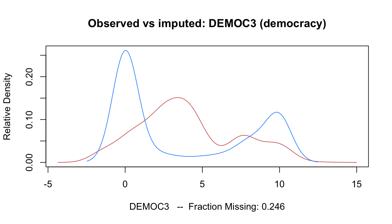
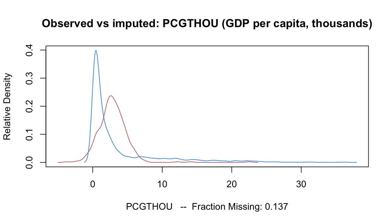
Imputed values (red density) should be broadly consistent with the observed distribution (black density). The same support and rough shape is expected; systematic divergence signals model misspecification. Note that small departures are expected and desirable — imputed values for DEMOC3 should reflect what we expect for countries where it is missing, which may genuinely differ from the observed distribution.

R

# DEMOC3: the key imputation target
plot(a.out, which.vars = "DEMOC3",
     main = "Observed vs imputed: DEMOC3 (democracy)")

# PCGTHOU: per capita GDP — check that imputed values are economically plausible
plot(a.out, which.vars = "PCGTHOU",
     main = "Observed vs imputed: PCGTHOU (GDP per capita, thousands)")

Tip

If imputed DEMOC3 values skew lower than observed values, this is consistent with the data-generating story: countries with missing democracy scores tend to be authoritarian, and Amelia’s imputation model — armed with the repression scores and temporal neighbours — correctly shifts the imputed distribution downward. This is a feature, not a bug.

Stata

* Overlay kernel densities of observed vs imputed DEMOC3 across imputations
mi convert wide, clear

local cmd ""
forvalues m = 1/20 {
    local cmd `cmd' (kdensity DEMOC3_`m', lcolor(red%20) lwidth(thin))
}
twoway (kdensity DEMOC3, lcolor(black) lwidth(medium) lpattern(solid)) ///
    `cmd', ///
    legend(order(1 "Observed" 2 "Imputed (m = 1..20)")) ///
    title("Density: observed vs imputed DEMOC3") xtitle("Democracy score")

mi convert mlong, clear   // restore long format for subsequent analysis

Over-imputation (model checking)

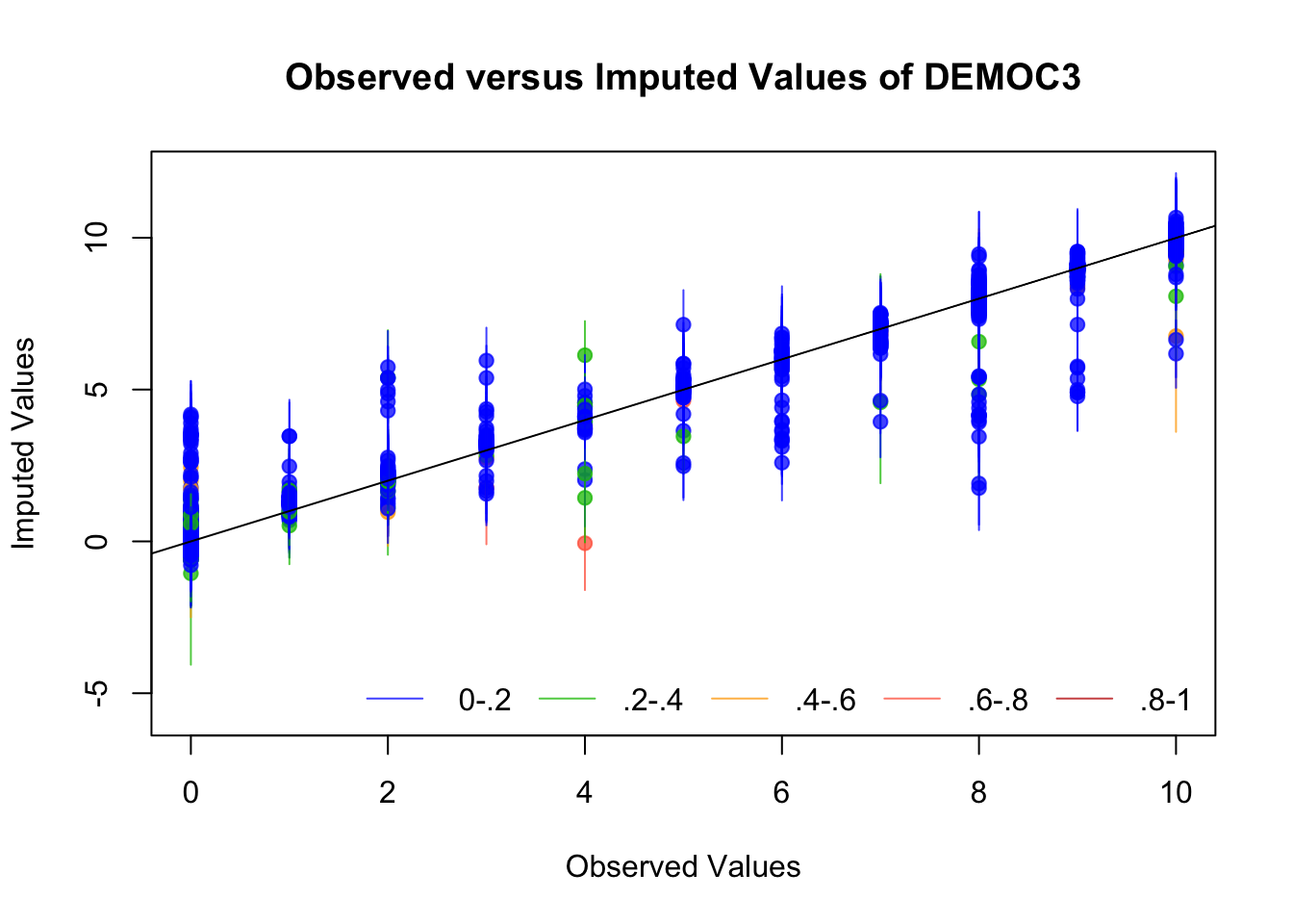
Over-imputation artificially sets observed values of DEMOC3 to missing, re-imputes them, and checks that the 90% imputation intervals cover the true observed values approximately 90% of the time. Systematic over- or under-coverage reveals model misspecification.

R

# This fits M imputations for each held-out observed value.
# Points are observed DEMOC3 values; vertical lines are 90% imputation intervals.
# Red = interval MISSES the true value; black = interval COVERS it.
overimpute(a.out, var = "DEMOC3")

Stata

* Over-imputation is not available in Stata's native mi suite.
*
* Recommended workflow: use R for imputation diagnostics, then export.
*
*   # In R:
*   overimpute(a.out, var = "DEMOC3")          # run diagnostic
*   write.amelia(a.out, file.stem = "isq99_imp",
*                format = "dta", original.data = TRUE)
*
* Then import the exported .dta files into Stata for analysis (see Section 9).

---

Panel Data Analysis

We now estimate the PTK model of state repression across all 20 imputed datasets and pool the results using Rubin’s combining rules. The theoretical model is:

\[\text{AINEW}_{it} = \alpha_i + \beta_1\,\text{AILAG}_{it} + \beta_2\,\text{DEMOC3}_{it} + \beta_3\,\text{MIL2}_{it} + \beta_4\,\text{LEFT}_{it} + \beta_5\,\text{CWARCOW}_{it} + \beta_6\,\text{IWARCOW2}_{it} + \beta_7\,\text{PCGTHOU}_{it} + \beta_8\,\text{PERCHPOP}_{it} + \varepsilon_{it}\]

where \(\alpha_i\) are country fixed effects (absorbed by the within transformation under FE, or modelled as random draws under RE). The coefficient \(\beta_2\) on DEMOC3 is the primary quantity of interest: Poe, Tate and Keith predict \(\beta_2 < 0\) — more democratic regimes repress less.

Warning

Lagged DV in fixed effects. Including AILAG in a fixed-effects estimator creates Nickell (1981) bias when \(T\) is small: the within-transformation introduces a mechanicial correlation between the transformed lagged outcome and the transformed residual, biasing \(\beta_1\) toward zero (and \(\beta_2\) away from it). This bias shrinks as \(T\) grows. We retain AILAG here following the PTK specification but note the issue for short panels.

Note

BRIT in FE models. BRIT (British colonial heritage) is time-invariant: it is absorbed entirely by country fixed effects and cannot be estimated under FE. It is included in the RE model, which exploits between-country variation.

Pooling helper function

R

The following function fits plm to each of the \(M\) imputed datasets, extracts coefficients and standard errors, and pools them using Rubin’s rules via mi.meld(). It also computes the Barnard–Rubin degrees of freedom and FMI per coefficient.

#' Pool plm estimates across Amelia imputations using Rubin's combining rules
#'
#' @param amelia_out  An object of class 'amelia' (output of amelia())
#' @param formula     Model formula passed to plm()
#' @param index       Panel index, e.g. c("IDORIGIN", "YEAR")
#' @param model       "within" (FE) or "random" (RE)
#' @param ...         Additional arguments passed to plm()
#' @return A tibble with pooled estimates, Rubin SE, B-R df, and FMI
pool_plm <- function(amelia_out, formula, index, model, ...) {

  # 1. Fit plm to each imputed dataset
  fits <- lapply(amelia_out$imputations, function(d) {
    plm(formula, data = d, index = index, model = model, ...)
  })

  # 2. Extract Q̂ (M × K) and SE (M × K)
  Q  <- do.call(rbind, lapply(fits, coef))
  SE <- do.call(rbind, lapply(fits, function(f) sqrt(diag(vcov(f)))))

  # 3. Rubin's combining rules via mi.meld()
  # mi.meld() returns 1×K matrices; as.numeric() drops the dimension
  pooled <- mi.meld(q = Q, se = SE)
  est    <- as.numeric(pooled$q.mi)
  se_mi  <- as.numeric(pooled$se.mi)

  # 4. Barnard-Rubin (1999) degrees of freedom and FMI
  M    <- nrow(Q)
  Ubar <- colMeans(SE^2)                   # within-imputation variance (Ū)
  B    <- apply(Q, 2, var)                 # between-imputation variance (B)
  T_   <- Ubar + (1 + 1/M) * B            # total variance (T)
  gamma <- (1 + 1/M) * B / T_             # fraction of missing information
  df_BR <- (M - 1) * (1 + Ubar / ((1 + 1/M) * B))^2

  # 5. Assemble tidy tibble
  tibble(
    term      = colnames(Q),
    estimate  = est,
    std.error = se_mi,
    statistic = est / se_mi,
    df        = df_BR,
    p.value   = 2 * pt(-abs(est / se_mi), df = df_BR),
    fmi       = gamma,
    W_var     = Ubar,
    B_var     = B,
    T_var     = T_
  )
}

Stata

* In Stata, mi estimate pools automatically — no helper function needed.
* It implements Rubin's combining rules and the Barnard-Rubin df adjustment.
*
* After mi estimate, Stata stores:
*   e(V_Ubar)  — within-imputation covariance matrix (Ū)
*   e(V_B)     — between-imputation covariance matrix (B)
*   e(V_Q)     — total (Rubin) covariance matrix (T)
*   e(fmi)     — fraction of missing information vector
*   e(df_mi)   — Barnard-Rubin degrees of freedom vector

Fixed-Effects Model

The within estimator eliminates all time-invariant confounding (including BRIT). The coefficient on DEMOC3 identifies the effect of within-country changes in democracy on repression.

R

# FE formula: exclude BRIT (time-invariant; dropped by FE anyway)
fe_formula <- AINEW ~ AILAG + DEMOC3 + MIL2 + LEFT +
              CWARCOW + IWARCOW2 + PCGTHOU + PERCHPOP

res_fe <- pool_plm(
  amelia_out = a.out,
  formula    = fe_formula,
  index      = c("IDORIGIN", "YEAR"),
  model      = "within"
)

res_fe |>
  select(term, estimate, std.error, statistic, df, p.value, fmi) |>
  gt() |>
  tab_header(
    title    = "Fixed-Effects Model — MI Pooled (M = 20)",
    subtitle = "Dependent variable: AINEW (physical integrity rights, AI scores)"
  ) |>
  fmt_number(columns = c(estimate, std.error, statistic, p.value, fmi),
             decimals = 4) |>
  fmt_number(columns = df, decimals = 1) |>
  cols_label(
    term      = "Coefficient",
    estimate  = "Q̄",
    std.error = "SE (Rubin)",
    statistic = "t",
    df        = "df (B–R)",
    p.value   = "p",
    fmi       = "FMI"
  ) |>
  tab_style(
    style     = cell_fill(color = "#fef9c3"),
    locations = cells_body(rows = p.value < 0.05)
  ) |>
  tab_footnote(
    footnote  = "FMI: fraction of missing information. Higher values = coefficient more sensitive to imputation model choices.",
    locations = cells_column_labels(columns = fmi)
  )

Fixed-Effects Model — MI Pooled (M = 20)
Dependent variable: AINEW (physical integrity rights, AI scores)
Coefficient	Q̄	SE (Rubin)	t	df (B–R)	p	FMI1
AILAG	0.4000	0.0263	15.2085	46.9	0.0000	0.6364
DEMOC3	−0.0462	0.0088	−5.2659	56.9	0.0000	0.5781
MIL2	0.0744	0.0728	1.0224	58.8	0.3108	0.5686
LEFT	0.0358	0.0761	0.4699	93.4	0.6395	0.4509
CWARCOW	0.4502	0.0760	5.9244	91.4	0.0000	0.4560
IWARCOW2	0.0738	0.0727	1.0150	90.0	0.3128	0.4594
PCGTHOU	−0.0130	0.0051	−2.5648	155.1	0.0113	0.3500
PERCHPOP	−0.0019	0.0036	−0.5281	259.0	0.5979	0.2709
1 FMI: fraction of missing information. Higher values = coefficient more sensitive to imputation model choices.

Stata

* ── Fixed-effects model ──────────────────────────────────────────────────────
* BRIT drops automatically under FE (time-invariant; absorbed by alpha_i)
mi estimate, dots notable: ///
    xtreg AINEW AILAG DEMOC3 MIL2 LEFT CWARCOW IWARCOW2 PCGTHOU PERCHPOP, fe

* notable option also prints between- and within-variance components
* mi estimate output includes:
*   - Pooled estimates (Q̄)
*   - Rubin standard errors (√T)
*   - Barnard-Rubin degrees of freedom per coefficient
*   - Fraction of missing information (FMI)

estimates store mi_fe

Random-Effects Model

The GLS random-effects estimator assumes \(\alpha_i \perp \mathbf{X}_{it}\) (random effects are uncorrelated with regressors). It is more efficient than FE when this assumption holds, and it allows estimation of time-invariant covariates like BRIT. The Mundlak test in Section 8 provides a formal assessment of the RE consistency assumption.

R

# RE formula: include BRIT (time-invariant, estimable under RE)
re_formula <- AINEW ~ AILAG + DEMOC3 + MIL2 + LEFT + BRIT +
              CWARCOW + IWARCOW2 + PCGTHOU + PERCHPOP

res_re <- pool_plm(
  amelia_out = a.out,
  formula    = re_formula,
  index      = c("IDORIGIN", "YEAR"),
  model      = "random"
)

res_re |>
  select(term, estimate, std.error, statistic, df, p.value, fmi) |>
  gt() |>
  tab_header(
    title    = "Random-Effects Model — MI Pooled (M = 20)",
    subtitle = "Dependent variable: AINEW (physical integrity rights, AI scores)"
  ) |>
  fmt_number(columns = c(estimate, std.error, statistic, p.value, fmi),
             decimals = 4) |>
  fmt_number(columns = df, decimals = 1) |>
  cols_label(
    term      = "Coefficient",
    estimate  = "Q̄",
    std.error = "SE (Rubin)",
    statistic = "t",
    df        = "df (B–R)",
    p.value   = "p",
    fmi       = "FMI"
  ) |>
  tab_style(
    style     = cell_fill(color = "#fef9c3"),
    locations = cells_body(rows = p.value < 0.05)
  )

Random-Effects Model — MI Pooled (M = 20)
Dependent variable: AINEW (physical integrity rights, AI scores)
Coefficient	Q̄	SE (Rubin)	t	df (B–R)	p	FMI
(Intercept)	1.0434	0.0678	15.3908	71.3	0.0000	0.5162
AILAG	0.6224	0.0198	31.4445	61.1	0.0000	0.5576
DEMOC3	−0.0307	0.0045	−6.8036	190.8	0.0000	0.3156
MIL2	0.1115	0.0399	2.7977	127.7	0.0059	0.3857
LEFT	−0.0807	0.0433	−1.8637	182.4	0.0640	0.3227
BRIT	−0.1178	0.0330	−3.5704	195.7	0.0004	0.3116
CWARCOW	0.5187	0.0659	7.8690	64.2	0.0000	0.5441
IWARCOW2	0.2148	0.0545	3.9392	166.7	0.0001	0.3376
PCGTHOU	−0.0159	0.0028	−5.7010	625.4	0.0000	0.1743
PERCHPOP	−0.0016	0.0038	−0.4395	200.9	0.6608	0.3075

Stata

* ── Random-effects model ─────────────────────────────────────────────────────
* BRIT is estimable under RE because it varies across units
mi estimate, dots notable: ///
    xtreg AINEW AILAG DEMOC3 MIL2 LEFT BRIT CWARCOW IWARCOW2 PCGTHOU PERCHPOP, re

estimates store mi_re

Complete-Case Comparison

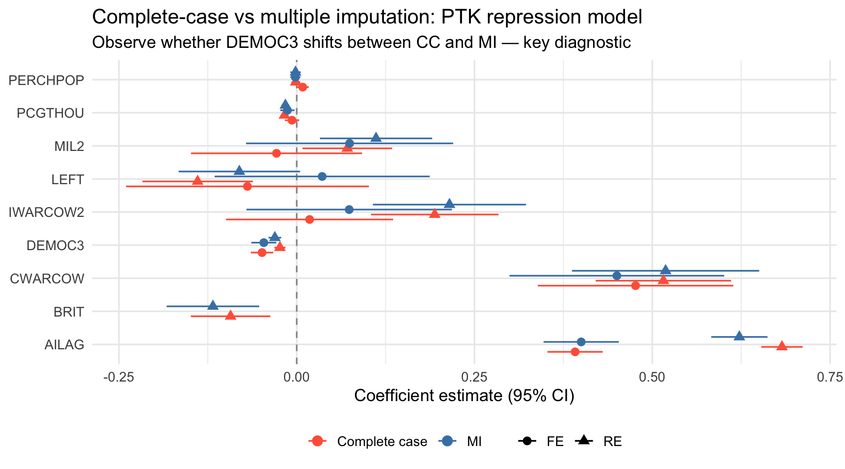
How much does listwise deletion distort our estimates? We fit the same models on the complete cases (observations with no missing values in any model variable) and plot all four estimator-method combinations side-by-side. The key comparison is the DEMOC3 coefficient, which is most directly affected by imputation.

R

# Complete-case data (listwise deletion)
cc_data <- ISQ99_Essex |>
  select(IDORIGIN, YEAR, AINEW, AILAG, DEMOC3, MIL2, LEFT, BRIT,
         CWARCOW, IWARCOW2, PCGTHOU, PERCHPOP) |>
  drop_na()

cat("Rows in full data:          ", nrow(ISQ99_Essex), "\n")

Rows in full data:           3222 

cat("Rows after listwise deletion:", nrow(cc_data), "\n")

Rows after listwise deletion: 2148 

cat("% observations lost:         ",
    round((1 - nrow(cc_data)/nrow(ISQ99_Essex))*100, 1), "%\n")

% observations lost:          33.3 %

# Complete-case FE
cc_fe_tidy <- plm(fe_formula, data = cc_data,
                  index = c("IDORIGIN", "YEAR"), model = "within") |>
  tidy(conf.int = TRUE) |>
  mutate(method = "Complete case – FE")

# Complete-case RE
cc_re_tidy <- plm(re_formula, data = cc_data,
                  index = c("IDORIGIN", "YEAR"), model = "random") |>
  tidy(conf.int = TRUE) |>
  mutate(method = "Complete case – RE")

# MI results with 95% CIs using Barnard-Rubin df
mi_fe_tidy <- res_fe |>
  mutate(
    conf.low  = estimate - qt(0.975, df) * std.error,
    conf.high = estimate + qt(0.975, df) * std.error,
    method    = "MI (Amelia H-K) – FE"
  )

mi_re_tidy <- res_re |>
  mutate(
    conf.low  = estimate - qt(0.975, df) * std.error,
    conf.high = estimate + qt(0.975, df) * std.error,
    method    = "MI (Amelia H-K) – RE"
  )

# Stack for plotting
plot_df <- bind_rows(
  cc_fe_tidy |> select(term, estimate, conf.low, conf.high, method),
  cc_re_tidy |> select(term, estimate, conf.low, conf.high, method),
  mi_fe_tidy |> select(term, estimate, conf.low, conf.high, method),
  mi_re_tidy |> select(term, estimate, conf.low, conf.high, method)
) |>
  mutate(
    estimator = if_else(str_detect(method, "FE"), "FE", "RE"),
    imputed   = if_else(str_detect(method, "MI"), "MI", "Complete case"),
    # Exclude the intercept term if present
    term = str_remove(term, "^\\(Intercept\\)")
  ) |>
  filter(term != "")

ggplot(plot_df,
       aes(x = estimate, y = term,
           colour = imputed, shape = estimator,
           xmin = conf.low, xmax = conf.high)) +
  geom_vline(xintercept = 0, linetype = "dashed", colour = "grey60") +
  geom_pointrange(position = position_dodge(width = 0.6), linewidth = 0.6) +
  scale_colour_manual(
    values = c("Complete case" = "tomato", "MI" = "steelblue"),
    name   = NULL
  ) +
  scale_shape_manual(values = c("FE" = 16, "RE" = 17), name = NULL) +
  labs(
    x        = "Coefficient estimate (95% CI)",
    y        = NULL,
    title    = "Complete-case vs multiple imputation: PTK repression model",
    subtitle = "Observe whether DEMOC3 shifts between CC and MI — key diagnostic"
  ) +
  theme_minimal(base_size = 13) +
  theme(legend.position = "bottom")

Stata

* ── Complete-case models ─────────────────────────────────────────────────────
xtreg AINEW AILAG DEMOC3 MIL2 LEFT CWARCOW IWARCOW2 PCGTHOU PERCHPOP, fe
estimates store cc_fe

xtreg AINEW AILAG DEMOC3 MIL2 LEFT BRIT CWARCOW IWARCOW2 PCGTHOU PERCHPOP, re
estimates store cc_re

* ── Coefficient comparison table ─────────────────────────────────────────────
* (requires estout: ssc install estout)
esttab cc_fe cc_re mi_fe mi_re,                              ///
    b(4) se(4) star(* 0.10 ** 0.05 *** 0.01)                 ///
    title("Complete-case vs MI estimates: PTK repression model")  ///
    mtitles("CC–FE" "CC–RE" "MI–FE" "MI–RE")                 ///
    note("Rubin SE for MI models. Barnard-Rubin df applied.")

* ── Coefficient plot ─────────────────────────────────────────────────────────
* (requires coefplot: ssc install coefplot)
coefplot (cc_fe, label("Complete case FE") msymbol(O) mcolor(tomato)) ///
         (mi_fe, label("MI FE")            msymbol(D) mcolor(navy)),    ///
    drop(_cons) xline(0) bycoefs                                         ///
    title("Complete-case vs MI: Fixed effects") legend(rows(1))

---

Variance Decomposition and Missing-Information Diagnostics

The between-imputation variance \(B\) and within-imputation variance \(\bar{U}\) diagnose qualitatively different problems:

• Large \(\bar{U}\), small \(B\): the sample is small or noisy; more data would help more than better imputation.
• Large \(B\), small \(\bar{U}\): coefficients are well-estimated within each imputed dataset but vary substantially across datasets — the imputed values are doing heavy lifting. Coefficients with this profile have high FMI and are most sensitive to imputation model choices.

For the PTK model, we expect DEMOC3 to show the highest FMI, reflecting both its missingness rate and its central role in the model.

R

bw_table <- bind_rows(
  res_fe |> mutate(model = "Fixed Effects"),
  res_re |> mutate(model = "Random Effects")
) |>
  select(model, term, W_var, B_var, T_var, fmi) |>
  mutate(
    pct_between = round(100 * B_var / T_var, 1),
    across(c(W_var, B_var, T_var), ~ round(.x, 6)),
    fmi = round(fmi, 4)
  )

bw_table |>
  gt(groupname_col = "model") |>
  tab_header(
    title    = "Between–Within Variance Decomposition (Rubin)",
    subtitle = "M = 20 imputations — PTK repression model"
  ) |>
  cols_label(
    term        = "Coefficient",
    W_var       = "Within (Ū)",
    B_var       = "Between (B)",
    T_var       = "Total (T)",
    fmi         = "FMI",
    pct_between = "% due to MI"
  ) |>
  tab_footnote(
    footnote  = "FMI = (1 + 1/M)B / T: fraction of total variance attributable to missing data.",
    locations = cells_column_labels(columns = fmi)
  ) |>
  tab_footnote(
    footnote  = "% due to MI = B/T × 100: share of total variance that comes from between-imputation variation.",
    locations = cells_column_labels(columns = pct_between)
  )

Between–Within Variance Decomposition (Rubin)
M = 20 imputations — PTK repression model
Coefficient	Within (Ū)	Between (B)	Total (T)	FMI1	% due to MI2
Fixed Effects
AILAG	0.000252	0.000419	0.000692	0.6364	60.6
DEMOC3	0.000033	0.000042	0.000077	0.5781	55.1
MIL2	0.002283	0.002866	0.005293	0.5686	54.2
LEFT	0.003184	0.002490	0.005798	0.4509	42.9
CWARCOW	0.003142	0.002508	0.005775	0.4560	43.4
IWARCOW2	0.002859	0.002314	0.005288	0.4594	43.8
PCGTHOU	0.000017	0.000009	0.000026	0.3500	33.3
PERCHPOP	0.000010	0.000003	0.000013	0.2709	25.8
Random Effects
(Intercept)	0.002223	0.002260	0.004596	0.5162	49.2
AILAG	0.000173	0.000208	0.000392	0.5576	53.1
DEMOC3	0.000014	0.000006	0.000020	0.3156	30.1
MIL2	0.000976	0.000584	0.001590	0.3857	36.7
LEFT	0.001269	0.000576	0.001873	0.3227	30.7
BRIT	0.000750	0.000323	0.001089	0.3116	29.7
CWARCOW	0.001981	0.002251	0.004345	0.5441	51.8
IWARCOW2	0.001969	0.000956	0.002973	0.3376	32.2
PCGTHOU	0.000006	0.000001	0.000008	0.1743	16.6
PERCHPOP	0.000010	0.000004	0.000014	0.3075	29.3
1 FMI = (1 + 1/M)B / T: fraction of total variance attributable to missing data.
2 % due to MI = B/T × 100: share of total variance that comes from between-imputation variation.

bind_rows(
  res_fe |> mutate(model = "FE"),
  res_re |> mutate(model = "RE")
) |>
  ggplot(aes(x = fmi, y = reorder(term, fmi), fill = model)) +
  geom_col(position = "dodge", width = 0.55) +
  geom_vline(xintercept = 0.3, linetype = "dashed", colour = "grey50") +
  scale_fill_manual(values = c("FE" = "steelblue", "RE" = "tomato"),
                    name   = "Model") +
  annotate("text", x = 0.31, y = 1, label = "FMI = 0.30\n(high sensitivity)",
           hjust = 0, size = 3, colour = "grey40") +
  labs(
    x        = "Fraction of missing information (FMI)",
    y        = NULL,
    title    = "Which coefficients are most sensitive to imputed values?",
    subtitle = "Higher FMI → estimate more dependent on imputation model specification"
  ) +
  theme_minimal(base_size = 13) +
  theme(legend.position = "bottom")

Stata

* ── Retrieve stored variance matrices after mi estimate ──────────────────────
mi estimate, dots: ///
    xtreg AINEW AILAG DEMOC3 MIL2 LEFT CWARCOW IWARCOW2 PCGTHOU PERCHPOP, fe

matrix W   = e(V_Ubar)    // within-imputation covariance (Ū)
matrix B   = e(V_B)       // between-imputation covariance (B)
matrix T   = e(V_Q)       // total (Rubin) covariance (T)
matrix fmi = e(fmi)       // vector of FMI values per coefficient

matrix list fmi

* Percent of total variance due to between-imputation variation
local M = 20
local k = colsof(fmi)
forvalues j = 1/`k' {
    scalar Bj    = B[`j', `j']
    scalar Tj    = T[`j', `j']
    scalar pct_j = Bj / Tj * 100
    display "Coefficient `j': pct_between = " pct_j
}

---

FE vs RE: The Hausman–Mundlak Test under Multiple Imputation

The standard Hausman (1978) test is a quadratic form in \(\hat{\beta}_\text{FE} - \hat{\beta}_\text{RE}\) and does not pool cleanly under Rubin’s rules, because the difference of two pooled estimators is not the same as the pooled difference. Two tractable alternatives exist.

Option A: Per-imputation Hausman tests

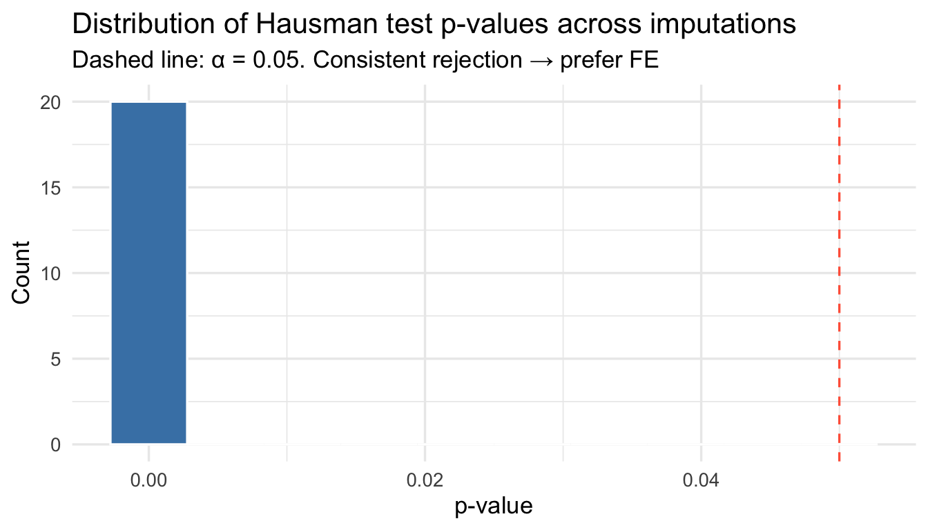
Run the Hausman test in each imputed dataset and inspect the distribution of \(\chi^2\) statistics or \(p\)-values. Consistent rejection across imputations is strong evidence against RE.

R

haus_stats <- lapply(seq_along(a.out$imputations), function(m) {
  d  <- a.out$imputations[[m]]
  fe <- plm(fe_formula, data = d, index = c("IDORIGIN", "YEAR"), model = "within")
  re <- plm(re_formula, data = d, index = c("IDORIGIN", "YEAR"), model = "random")
  ht <- phtest(fe, re)
  tibble(m = m, statistic = ht$statistic, p.value = ht$p.value, df = ht$parameter)
})

haus_df <- bind_rows(haus_stats)

haus_df |>
  summarise(
    mean_chi2  = round(mean(statistic), 3),
    sd_chi2    = round(sd(statistic), 3),
    pct_reject = round(mean(p.value < 0.05) * 100, 1)
  ) |>
  gt() |>
  tab_header(
    title    = "Hausman test across M = 20 imputations",
    subtitle = "H₀: RE is consistent (random effects uncorrelated with regressors)"
  ) |>
  cols_label(
    mean_chi2  = "Mean χ²",
    sd_chi2    = "SD χ²",
    pct_reject = "% reject at α = 0.05"
  )

Hausman test across M = 20 imputations
H₀: RE is consistent (random effects uncorrelated with regressors)
Mean χ²	SD χ²	% reject at α = 0.05
660.206	79.116	100

ggplot(haus_df, aes(x = p.value)) +
  geom_histogram(bins = 10, fill = "steelblue", colour = "white") +
  geom_vline(xintercept = 0.05, linetype = "dashed", colour = "tomato") +
  labs(
    x        = "p-value",
    y        = "Count",
    title    = "Distribution of Hausman test p-values across imputations",
    subtitle = "Dashed line: α = 0.05. Consistent rejection → prefer FE"
  ) +
  theme_minimal(base_size = 13)

Stata

* ── Per-imputation Hausman tests ─────────────────────────────────────────────
local reject = 0
forvalues m = 1/20 {
    quietly xtreg AINEW AILAG DEMOC3 MIL2 LEFT CWARCOW IWARCOW2 ///
        PCGTHOU PERCHPOP if _mi_m == `m', fe
    estimates store fe_`m'
    quietly xtreg AINEW AILAG DEMOC3 MIL2 LEFT BRIT CWARCOW IWARCOW2 ///
        PCGTHOU PERCHPOP if _mi_m == `m', re
    estimates store re_`m'
    quietly hausman fe_`m' re_`m'
    if r(p) < 0.05 local reject = `reject' + 1
    display "m = `m': chi2 = " r(chi2) "   p = " r(p)
}
display "Imputations rejecting H0 at 5%: `reject' / 20"

Option B: Mundlak Device (Recommended)

The Mundlak (1978) device adds the within-unit means of all time-varying regressors to the RE specification. The RE–FE choice becomes a test of whether these group means are jointly zero — a linear restriction that pools straightforwardly under Rubin’s rules. The joint test below uses the D2 statistic of Li, Meng, Raghunathan & Rubin (1991), which pools the \(M\) per-imputation Wald chi-squared statistics into a single \(F\) reference distribution.

R

# Compute group means within each imputed dataset and add to the data.
# Group means of time-varying continuous covariates capture the "between"
# variation that distinguishes FE from RE.
add_group_means <- function(d) {
  d |>
    group_by(IDORIGIN) |>
    mutate(
      m_DEMOC3   = mean(DEMOC3,   na.rm = TRUE),
      m_PCGTHOU  = mean(PCGTHOU,  na.rm = TRUE),
      m_PERCHPOP = mean(PERCHPOP, na.rm = TRUE)
    ) |>
    ungroup()
}

a_mundlak <- a.out
a_mundlak$imputations <- lapply(a.out$imputations, add_group_means)

# RE model augmented with group means — the Mundlak (1978) specification
mundlak_formula <- AINEW ~ AILAG + DEMOC3 + MIL2 + LEFT + BRIT +
                   CWARCOW + IWARCOW2 + PCGTHOU + PERCHPOP +
                   m_DEMOC3 + m_PCGTHOU + m_PERCHPOP

res_mundlak <- pool_plm(
  amelia_out = a_mundlak,
  formula    = mundlak_formula,
  index      = c("IDORIGIN", "YEAR"),
  model      = "random"
)

res_mundlak |>
  select(term, estimate, std.error, statistic, df, p.value) |>
  mutate(
    role = if_else(str_starts(term, "m_"), "Mundlak term (between-unit)", "Structural")
  ) |>
  gt(groupname_col = "role") |>
  tab_header(
    title    = "Mundlak (1978) RE model — MI Pooled (M = 20)",
    subtitle = "H₀: group-mean coefficients = 0 ↔ RE is consistent"
  ) |>
  fmt_number(columns = c(estimate, std.error, statistic, p.value), decimals = 4) |>
  fmt_number(columns = df, decimals = 1) |>
  tab_style(
    style     = cell_fill(color = "#fef9c3"),
    locations = cells_body(rows = p.value < 0.05)
  ) |>
  tab_footnote(
    footnote  = "Mundlak terms are the within-country means of each time-varying covariate. Significant terms indicate that between-unit variation drives the coefficient, favouring FE.",
    locations = cells_row_groups(groups = "Mundlak term (between-unit)")
  )

Mundlak (1978) RE model — MI Pooled (M = 20)
H₀: group-mean coefficients = 0 ↔︎ RE is consistent
term	estimate	std.error	statistic	df	p.value
Structural
(Intercept)	1.0574	0.0861	12.2865	58.2	0.0000
AILAG	0.6201	0.0202	30.6549	57.7	0.0000
DEMOC3	−0.0311	0.0088	−3.5531	57.5	0.0008
MIL2	0.1060	0.0401	2.6404	124.6	0.0093
LEFT	−0.0834	0.0466	−1.7896	120.6	0.0760
BRIT	−0.1213	0.0352	−3.4478	142.5	0.0007
CWARCOW	0.5159	0.0662	7.7891	63.3	0.0000
IWARCOW2	0.2167	0.0546	3.9682	164.0	0.0001
PCGTHOU	−0.0080	0.0052	−1.5318	205.1	0.1271
PERCHPOP	−0.0020	0.0038	−0.5372	301.6	0.5915
Mundlak term (between-unit)1
m_DEMOC3	0.0018	0.0112	0.1591	52.8	0.8742
m_PCGTHOU	−0.0117	0.0062	−1.8658	260.3	0.0632
m_PERCHPOP	0.0018	0.0170	0.1057	54.1	0.9162
1 Mundlak terms are the within-country means of each time-varying covariate. Significant terms indicate that between-unit variation drives the coefficient, favouring FE.

# ── D2 pooled test (Li, Meng, Raghunathan & Rubin 1991, Stat. Sin. 1:65-92) ─
#
# Per-imputation Wald chi-squared statistics W_1,...,W_M for k restrictions
# are pooled as:
#
#   W̄  = mean(W_m)
#   b   = var(W_m)
#   r2  = (1 + 1/M) * b / (2k)      # between-imputation variance relative
#                                    # to chi2(k) null variance = 2k
#   D2  = (W̄/k - r2) / (1 + r2)    ~ F(k, v2)
#   v2  = (M - 1) * (1 + 1/r2)²
#
# When r2 → 0 (no MI uncertainty), v2 → ∞ and D2 ≈ chi2(k)/k (standard).
# When r2 → ∞ (MI dominates), v2 → M - 1 (dominated by imputation variance).

d2_test <- function(chi2_vals, k) {
  M    <- length(chi2_vals)
  Wbar <- mean(chi2_vals)
  b    <- var(chi2_vals)

  r2 <- (1 + 1/M) * b / (2 * k)
  D2 <- (Wbar / k - r2) / (1 + r2)

  v2 <- if (r2 < .Machine$double.eps * 100) Inf else (M - 1) * (1 + 1/r2)^2
  p  <- pf(D2, df1 = k, df2 = v2, lower.tail = FALSE)

  tibble(D2 = D2, df1 = k, df2 = v2, p.value = p,
         r2 = r2, chi2_bar = Wbar, chi2_var = b, M = M)
}

# Per-imputation Wald chi-squared for H0: m_DEMOC3 = m_PCGTHOU = m_PERCHPOP = 0
mundlak_terms <- c("m_DEMOC3", "m_PCGTHOU", "m_PERCHPOP")
k             <- length(mundlak_terms)

chi2_vals <- vapply(a_mundlak$imputations, function(d) {
  fit  <- plm(mundlak_formula, data = d,
              index = c("IDORIGIN", "YEAR"), model = "random")
  bvec <- coef(fit)[mundlak_terms]
  Vmat <- vcov(fit)[mundlak_terms, mundlak_terms]
  as.numeric(t(bvec) %*% solve(Vmat) %*% bvec)
}, numeric(1))

cat(sprintf(
  "Per-imputation Wald chi2(%d): mean = %.3f  SD = %.3f  range = [%.3f, %.3f]\n",
  k, mean(chi2_vals), sd(chi2_vals), min(chi2_vals), max(chi2_vals)
))

Per-imputation Wald chi2(3): mean = 8.013  SD = 3.855  range = [2.762, 20.926]

d2_result <- d2_test(chi2_vals, k = k)

d2_result |>
  gt() |>
  tab_header(
    title    = "D2 Pooled Test — Joint Significance of Mundlak Terms",
    subtitle = "H₀: m_DEMOC3 = m_PCGTHOU = m_PERCHPOP = 0 (RE is consistent with FE)"
  ) |>
  fmt_number(columns = c(D2, r2, chi2_bar, chi2_var), decimals = 4) |>
  fmt_number(columns = df2, decimals = 1) |>
  fmt_number(columns = p.value, decimals = 4) |>
  cols_label(
    D2       = "D₂",
    df1      = "df₁ (k)",
    df2      = "df₂ (v₂)",
    p.value  = "p",
    r2       = "r₂",
    chi2_bar = "W̄",
    chi2_var = "Var(W)",
    M        = "M"
  ) |>
  tab_footnote(
    footnote  = "r₂ = (1 + 1/M)·Var(W)/(2k): relative between-imputation variance of the test statistic.",
    locations = cells_column_labels(columns = r2)
  ) |>
  tab_footnote(
    footnote  = "v₂ = (M − 1)(1 + 1/r₂)²: effective denominator df; shrinks toward M − 1 as MI uncertainty grows.",
    locations = cells_column_labels(columns = df2)
  )

D2 Pooled Test — Joint Significance of Mundlak Terms
H₀: m_DEMOC3 = m_PCGTHOU = m_PERCHPOP = 0 (RE is consistent with FE)
D₂	df₁ (k)	df₂ (v₂)1	p	r₂2	W̄	Var(W)	M
0.0196	3	36.4	0.9962	2.6004	8.0133	14.8594	20
1 v₂ = (M − 1)(1 + 1/r₂)²: effective denominator df; shrinks toward M − 1 as MI uncertainty grows.
2 r₂ = (1 + 1/M)·Var(W)/(2k): relative between-imputation variance of the test statistic.

Stata

* ── Mundlak device ───────────────────────────────────────────────────────────
* mi passive computes group means within each imputed dataset automatically.
* This is the key advantage over a manual loop — Stata propagates the
* computation to all _mi_m > 0 datasets.

mi passive: bysort IDORIGIN: egen m_DEMOC3   = mean(DEMOC3)
mi passive: bysort IDORIGIN: egen m_PCGTHOU  = mean(PCGTHOU)
mi passive: bysort IDORIGIN: egen m_PERCHPOP = mean(PERCHPOP)

* Augmented RE model
mi estimate, dots notable: ///
    xtreg AINEW AILAG DEMOC3 MIL2 LEFT BRIT CWARCOW IWARCOW2 PCGTHOU PERCHPOP ///
          m_DEMOC3 m_PCGTHOU m_PERCHPOP, re

* ── D2 pooled joint test (Li et al. 1991) ────────────────────────────────────
* Stata's mi test implements the D2 statistic automatically after mi estimate.
* It computes per-imputation Wald statistics and pools them as:
*     D2 = (W̄/k - r2) / (1 + r2)  ~  F(k, v2)
* where r2 = (1 + 1/M) * Var(W_m) / (2k) and v2 = (M-1)(1 + 1/r2)^2.

mi test m_DEMOC3 m_PCGTHOU m_PERCHPOP

* Output includes D2, numerator df (k = 3), denominator df (v2), and p-value.
*   Significant  →  group means ≠ 0  →  prefer FE (RE inconsistent)
*   Insignificant →  cannot reject that RE is consistent; prefer RE for efficiency
*
* r2 is stored in r(r2) after mi test for inspection.

---

Exporting Amelia Imputations to Stata

If you prefer to impute in R (using Amelia’s TSCS features) and analyse in Stata (using Stata’s mi estimate and post-estimation suite), write.amelia() exports all imputed datasets as .dta files.

R

# Export: creates isq99_imp0.dta (original data) and
#         isq99_imp1.dta … isq99_imp20.dta (imputed datasets)
write.amelia(a.out,
             file.stem     = "isq99_imp",
             format        = "dta",
             original.data = TRUE)

Stata

* ── Import Amelia imputations into Stata's mi framework ──────────────────────
* Run after write.amelia() in R produces isq99_imp0.dta ... isq99_imp20.dta

* Option A — manual append then mi import flong
clear
gen _mi_m = .
forvalues m = 0/20 {
    append using isq99_imp`m'.dta
    replace _mi_m = `m' if _mi_m == .
}

* Declare as mi data in flong format (one imputed dataset stacked per _mi_m value)
mi import flong, m(_mi_m) id(IDORIGIN YEAR)
xtset IDORIGIN YEAR

* ── Replicate FE and RE analyses from R ──────────────────────────────────────
mi estimate, dots: ///
    xtreg AINEW AILAG DEMOC3 MIL2 LEFT CWARCOW IWARCOW2 PCGTHOU PERCHPOP, fe

mi estimate, dots: ///
    xtreg AINEW AILAG DEMOC3 MIL2 LEFT BRIT CWARCOW IWARCOW2 PCGTHOU PERCHPOP, re

---

Summary and Recommended Workflow

This document illustrates a complete workflow for multiple imputation of a TSCS human rights panel, structured around the core insights of Honaker and King (2010).

1. Diagnose missingness — use vis_dat(), vis_miss(), gg_miss_var(), and the temporal heatmap to understand where data are missing. Check whether the spatial/temporal pattern is consistent with MAR.

2. Make the MAR case — in TSCS human rights data, temporal neighbours of a missing democracy score (and co-observed variables like repression itself, political rights, and economic indicators) provide strong proxies for the unobserved value. This makes MAR far more defensible than MCAR.

3. Specify the imputation model — use polytime = 2 to add a quadratic time trend in each imputation equation (the core H-K innovation). Add lags and leads for key time-varying predictors to exploit AR structure. Use intercs = TRUE for unit-specific trends if the panel is small enough; fall back to intercs = FALSE for large panels. Declare ords and noms correctly.

4. Choose \(M\) — a common heuristic is \(M \approx\) percentage of missing cases (Bodner 2008, White et al. 2011). With moderate missingness in DEMOC3, \(M = 20\) is a reasonable starting point.

5. Check diagnostics — density overlap should show imputed democracy values shifted toward lower scores relative to observed (consistent with the selection story). Over-imputation coverage near 90% confirms the model. Systematic failures signal misspecification.

6. Pool with Rubin’s rules — use mi.meld() in R or mi estimate in Stata. Report FMI alongside standard errors. Coefficients with FMI > 0.30 (particularly DEMOC3) are sensitive to imputation model choices and deserve robustness checks.

7. Test FE vs RE — use the Mundlak device and D2 pooled test (mi test in Stata), not the raw Hausman statistic. The Mundlak approach produces a linear restriction that pools correctly under Rubin’s rules.

Key References

• Honaker, J. & King, G. (2010). What to Do about Missing Values in Time-Series Cross-Section Data. American Journal of Political Science, 54(2), 561–581.
• King, G., Honaker, J., Joseph, A. & Scheve, K. (2001). Analyzing Incomplete Political Science Data: An Alternative Algorithm for Multiple Imputation. American Political Science Review, 95(1), 49–69.
• Honaker, J., King, G. & Blackwell, M. (2011). Amelia II: A Program for Missing Data. Journal of Statistical Software, 45(7), 1–47.
• Poe, S.C., Tate, C.N. & Keith, L.C. (1999). Repression of the Human Right to Personal Integrity Revisited: A Global Cross-National Study Covering the Years 1976–1993. International Studies Quarterly, 43(2), 291–313.
• Rubin, D.B. (1987). Multiple Imputation for Nonresponse in Surveys. Wiley.
• Li, K.H., Meng, X.L., Raghunathan, T.E. & Rubin, D.B. (1991). Significance Levels from Repeated p-Values with Multiply-Imputed Data. Statistica Sinica, 1(1), 65–92.
• Barnard, J. & Rubin, D.B. (1999). Small-Sample Degrees of Freedom with Multiple Imputation. Biometrika, 86(4), 948–955.
• Mundlak, Y. (1978). On the Pooling of Time Series and Cross Section Data. Econometrica, 46(1), 69–85.
• Nickell, S. (1981). Biases in Dynamic Models with Fixed Effects. Econometrica, 49(6), 1417–1426.
• Bodner, T.E. (2008). What Improves with Increased Missing Data Imputations? Structural Equation Modeling, 15(4), 651–675.
• Hausman, J.A. (1978). Specification Tests in Econometrics. Econometrica, 46(6), 1251–1271.

---

A Postscript on Recent Developments and on Imputing Outcomes

The state of the art in Multiple Imputation (MI) for missing outcome variables (\(Y\)) reflects a nuanced consensus: imputing outcomes is not always necessary or beneficial, but when done correctly, it preserves statistical validity, prevents bias in covariates, and maximizes power.

The handling of missing outcome variables (\(Y\)) in statistical modeling presents a well-known methodological divergence between cross-sectional and panel data structures. In standard cross-sectional research, the prevailing consensus under Missing at Random (MAR) assumptions often favors Complete Case Analysis (CCA) or “Impute-Then-Delete” (MID) strategies over outcome imputation. When missingness is confined strictly to the dependent variable and covariates (\(X\)) are fully observed, imputing \(Y\) from \(X\) alone adds no new information to the regression model; it merely introduces Monte Carlo simulation noise without reducing parameter variance or bias.

However, in Panel and Time-Series Cross-Sectional (TSCS) data—where units \(i = 1, \dots, N\) are observed repeatedly across time periods \(t = 1, \dots, T\)—this cross-sectional logic breaks down. Panel structures contain deep temporal persistence and cross-sectional dependencies. An outcome missing at time \(t\) (\(Y_{it}\)) is bound by observed historical records (\(Y_{i,t-1}, Y_{i,t-2}\)) and future realizations (\(Y_{i,t+1}, Y_{i,t+2}\)), as well as contemporaneous outcomes from correlated units (\(Y_{jt}\)).

In this context, past and future realizations of the outcome function as exceptionally powerful auxiliary variables. Including these temporal proxies into an imputation model drastically reduces variance, enhances statistical power, and transforms plausible Missing Not at Random (MNAR) mechanisms into manageable MAR mechanisms. Consequently, outcome imputation in panel data is not merely permissible—it is often indispensable for valid inference.

This document synthesizes the methodological evolution of panel outcome imputation, taking the foundational work of Honaker and King (2010) as a starting point and tracing subsequent frontiers through matrix completion, substantive model compatibility, and non-parametric machine learning.

---

The Foundational Baseline: Honaker & King (2010)

The Expectation-Maximization with Bootstrapping (EMb) Framework

Prior to Honaker and King (2010), applied panel researchers routinely resorted to listwise deletion or basic interpolation, both of which severely distort time-series dynamics and standard errors. Honaker and King established a rigorous Bayesian multiple imputation framework designed specifically for TSCS data, implemented in the Amelia II algorithm.

The model assumes that the complete data \(D = (X, Y)\) follow a Multivariate Normal (MVN) distribution:

\[D_{it} \sim \mathcal{N}_p(\boldsymbol{\mu}, \boldsymbol{\Sigma})\]

To capture the spatio-temporal structure intrinsic to panel data without triggering the “curse of dimensionality” (which occurs if fixed effects are estimated for every unit and time period in large panels), Honaker and King introduced two critical innovations:

1. Smooth Time Trends via Polynomials and Splines: Time dynamics are incorporated by modeling unit trajectories as smooth functions of time, \(f(t)\), using orthogonal polynomials or cubic splines: \[D_{it} \sim \mathcal{N}_p(\boldsymbol{\mu}_i + f(t), \boldsymbol{\Sigma})\]
2. Prior Distributions on Individual Cell Values: Priors allow researchers to incorporate domain knowledge or explicit observation-level uncertainties, stabilizing the Expectation-Maximization (EM) algorithm under sparse data conditions.

The Role of \(Y_{it}\) as an Auxiliary Target

Honaker and King demonstrated that when imputing \(Y_{it}\), the presence of leads (\(Y_{i,t+1}\)) and lags (\(Y_{i,t-1}\)) in the imputation model fundamentally alters the information matrix. Under the MVN setup, the conditional expectation of a missing outcome \(Y_{it}\) given observed history takes the form of a dynamic linear filter:

\[\mathbb{E}[Y_{it} \mid D_{\text{obs}}] = \alpha_i + \sum_{k=1}^K \gamma_k Y_{i,t-k} + \sum_{m=1}^M \delta_m Y_{i,t+m} + \boldsymbol{\beta}^T X_{it} + f(t)\]

Because the auto-correlation \(\text{Corr}(Y_{it}, Y_{i,t-1})\) in panel data typically ranges between \(0.6\) and \(0.95\), the conditional variance \(\text{Var}(Y_{it} \mid D_{\text{obs}})\) shrinks dramatically compared to cross-sectional settings. This high predictive accuracy validates outcome imputation in TSCS environments.

Limitations of the MVN Paradigm

Despite its widespread adoption, the Honaker-King framework exhibits three major theoretical limitations:

• Linearity and Normality Assumptions: MVN models struggle with non-linear trajectories, bounded outcomes, count data, or discrete panel indicators (e.g., binary regime changes).
• Model Incompatibility in Dynamic Regressions: Imputing \(Y_{it}\) under joint normality independently of the user’s substantive analysis model (such as an autoregressive fixed-effects regression) induces attenuation bias in estimated lag coefficients (\(\hat{\rho}\)).
• Curse of Latent Dimensionality: While smooth time trends handle deterministic trajectories well, they fail to capture unobserved, time-varying latent factors that affect multiple units simultaneously.

---

Frontier 1: Matrix Completion & Causal Panel Inference

Re-framing Missing Outcomes as Counterfactuals

A major modern advance shifts the conceptualization of panel outcome imputation from missing data mechanics to causal inference under potential outcomes. Developed by Athey, Bayati, Doudchenko, Imbens, and Khosravi (2021) and extended by Liu, Wang, and Xu (2023), this framework models panel causal estimation (e.g., Difference-in-Differences, Synthetic Control) explicitly as an outcome imputation problem over an \(N \times T\) matrix \(\mathbf{Y}\).

Let \(\mathbf{Y}\) be an \(N \times T\) matrix where entry \(Y_{it}\) represents the observed outcome. Under a staggered treatment adoption design:

\[Y_{it} = \begin{cases} Y_{it}(0) & \text{if unit } i \text{ is untreated at time } t \\ Y_{it}(1) & \text{if unit } i \text{ is treated at time } t \end{cases}\]

For all treated unit-periods, the untreated potential outcome \(Y_{it}(0)\) is missing by definition. Estimating the Average Treatment Effect on the Treated (ATT) is therefore mathematically equivalent to imputing the missing entries in the \(N \times T\) matrix \(\mathbf{Y}(0)\).

T_1 T_2 T_3 T_4 … T_T N_1 [ Y Y Y Y … Y ] <- Fully Observed Control Unit N_2 [ Y Y Y ? … ? ] <- Treatment at T_4 (Missing Potential Outcomes) N_3 [ Y ? ? ? … ? ] <- Treatment at T_2 (Missing Potential Outcomes) … N_N [ Y Y Y Y … Y ]

Nuclear-Norm Regularization and Interactive Fixed Effects

Rather than specifying parametric time polynomials \(f(t)\) as in Amelia II, Matrix Completion decomposes the outcome matrix \(\mathbf{Y}(0)\) into a low-rank matrix \(\mathbf{L}\) capturing unobserved unit factors and time trends, plus a sparse matrix \(\mathbf{S}\) and noise \(\mathbf{E}\):

\[\mathbf{Y}(0) = \mathbf{L} + \mathbf{S} + \mathbf{E}\]

The low-rank component \(\mathbf{L}\) generalizes traditional Two-Way Fixed Effects (TWFE) by representing outcomes as interactive fixed effects:

\[L_{it} = \alpha_i + \xi_t + \boldsymbol{\gamma}_i^T \boldsymbol{\lambda}_t\]

where \(\boldsymbol{\gamma}_i\) is a vector of unobserved unit factor loadings and \(\boldsymbol{\lambda}_t\) is a vector of unobserved time factors.

The missing elements of \(\mathbf{Y}(0)\) are imputed by solving a convex optimization problem with a nuclear-norm penalty on \(\mathbf{L}\):

\[\hat{\mathbf{L}} = \arg\min_{\mathbf{L}} \left\{ \frac{1}{|\Omega|} \sum_{(i,t) \in \Omega} (Y_{it} - L_{it})^2 + \lambda \|\mathbf{L}\|_* \right\}\]

where \(\Omega\) is the set of observed (untreated) unit-periods, and \(\|\mathbf{L}\|_* = \sum_{k} \sigma_k(\mathbf{L})\) denotes the nuclear norm (the sum of singular values of \(\mathbf{L}\)).

Methodological Strengths

1. Non-Parametric Flexibility: Learns complex, unobserved time-varying factor structures across units without requiring manual specification of lead/lag structures.
2. Robustness to High-Dimensional Missingness: Performs exceptionally well in Large \(N\), Large \(T\) settings where large blocks of outcomes are missing or unobserved.

---

Frontier 2: Substantive Model Compatible FCS (Panel SMC-FCS)

The Incompatibility Problem in Dynamic Panel Regressions

When researchers estimate dynamic panel specifications containing both unit fixed effects and lagged dependent variables—such as the standard Arellano-Bond setup:

\[Y_{it} = \rho Y_{i,t-1} + \boldsymbol{\beta}^T X_{it} + \alpha_i + \varepsilon_{it}\]

standard Fully Conditional Specification (FCS / MICE) and MVN imputation algorithms (including Amelia II) produce severely biased estimates of \(\rho\).

This bias stems from imputation model incompatibility. Standard MICE constructs a linear conditional model for \(Y_{it}\) given \(Y_{i,t-1}, Y_{i,t+1}, X_{it}\). However, the true mathematical distribution of \(Y_{it}\) conditional on \(Y_{i,t-1}\) and \(Y_{i,t+1}\) derived from the substantive equation above is non-linear and constrained by \(\alpha_i\). Standard MI models fail to preserve this structural identity, forcing the imputed draws of \(Y_{it}\) to attenuate toward the unconditional mean. Consequently, the estimated dynamic persistence parameter \(\hat{\rho}\) is biased downward (attenuation bias).

Theoretical Mechanics of SMC-FCS

Substantive Model Compatible Fully Conditional Specification (SMC-FCS), pioneered by Bartlett et al. (2015) and extended to panel structures, resolves incompatibility by ensuring the imputation model for any variable is formally derived from the substantive analysis model \(f(Y_{it} \mid X_{it}, \boldsymbol{\theta})\).

Instead of posing an arbitrary linear imputation model for a missing outcome or covariate \(Z\), SMC-FCS uses Bayes’ theorem to decompose the conditional density:

\[p(Z \mid \text{others}, \boldsymbol{\theta}) \propto p(\text{Substantive Outcome} \mid Z, \text{covariates}, \boldsymbol{\theta}_1) \times p(Z \mid \text{auxiliary covariates}, \boldsymbol{\theta}_2)\]

For a dynamic panel model where \(Y_{it}\) is missing, the target draw for \(Y_{it}^*\) must simultaneously satisfy two substantive constraints: 1. It must serve as the outcome at time \(t\) given past states: \(p(Y_{it} \mid Y_{i,t-1}, X_{it}, \alpha_i)\). 2. It must serve as the lagged predictor for the observed outcome at time \(t+1\): \(p(Y_{i,t+1} \mid Y_{it}, X_{i,t+1}, \alpha_i)\).

The SMC-FCS draw for \(Y_{it}\) evaluates the joint likelihood:

\[p(Y_{it}^* \mid \cdot) \propto \exp \left( -\frac{(Y_{it} - \rho Y_{i,t-1} - \boldsymbol{\beta}^T X_{it} - \alpha_i)^2}{2\sigma_{\varepsilon}^2} - \frac{(Y_{i,t+1} - \rho Y_{it} - \boldsymbol{\beta}^T X_{i,t+1} - \alpha_i)^2}{2\sigma_{\varepsilon}^2} \right)\]

By sampling from this exact structural density (using Metropolis-Hastings steps within MICE chains), Panel SMC-FCS eliminates attenuation bias in autoregressive terms and maintains the exact covariance structure demanded by dynamic panel estimators.

---

Frontier 3: Multilevel FCS & Non-Parametric Machine Learning

Micro-Panels and Multilevel MICE (jomo)

In micro-panels characterized by large \(N\) (\(10^3 - 10^5\) individuals) and small \(T\) (\(3 - 10\) waves), assumptions of multivariate normality across time vectors break down, particularly when outcomes are binary, ordinal, or count variables (e.g., employment status, health indicators).

Multilevel FCS, implemented in packages such as jomo (Quartagno & Carpenter, 2016) and mice.impute.2l.pan, explicitly decomposes outcome variation into within-individual (Level 1) and between-individual (Level 2) components using Generalized Linear Mixed Models (GLMMs):

\[Y_{it} = \boldsymbol{\beta}^T X_{it} + \mathbf{u}_i^T \mathbf{Z}_{it} + \varepsilon_{it}\]

\[\mathbf{u}_i \sim \mathcal{N}(\mathbf{0}, \boldsymbol{\Omega})\]

When \(Y_{it}\) is binary or categorical, a probit or logit link function is applied within the Level-1 stage:

\[\mathbb{P}(Y_{it} = 1 \mid X_{it}, \mathbf{u}_i) = g^{-1}(\boldsymbol{\beta}^T X_{it} + \mathbf{u}_i^T \mathbf{Z}_{it})\]

Imputations for missing discrete outcomes \(Y_{it}\) are sampled directly from the latent continuous representation under the estimated random-effects covariance structure \(\boldsymbol{\Omega}\), ensuring proper variance estimation across waves without violating distributional bounds.

Non-Parametric Panel Machine Learning (missForest and Ensembles)

For panel datasets featuring complex non-linear trajectories, structural breaks, or high-dimensional interactions among covariates, parametric mixed models become intractable. Non-parametric ensemble methods—most notably Random Forest imputation via missForest (Stekhoven & Bühlmann, 2012) adapted for panel structures—have emerged as state-of-the-art tools.

To adapt tree-based algorithms for panel outcome imputation, time indices and temporal aggregations are explicitly embedded into the feature space:

\[F_{it} = \left[ X_{it}, \; Y_{i,t-1}, \; Y_{i,t+1}, \; \bar{Y}_i, \; \sigma(Y_i), \; f(t) \right]\]

where \(\bar{Y}_i\) is the unit-level historical mean and \(\sigma(Y_i)\) is the unit-level standard deviation.

Advantages of Machine Learning Imputation

• Captures Arbitrary Interactions: Trees automatically split on time steps and unit characteristics, isolating subgroup-specific trajectories without requiring explicit interaction terms.
• Handles Mixed Outcome Types: Seamlessly imputes continuous, binary, and multi-category outcomes within the same panel framework.

Methodological Caution on Variance Estimation

While tree ensembles achieve superior predictive accuracy (minimizing Root Mean Squared Error for missing entries), standard bootstrapping of ML models often underestimates the total variance of imputed datasets. For hypothesis testing, ML outcome imputation must be paired with Rubin’s rules using enlarged imputation numbers (\(M \ge 50\)) or generalized synthetic donor matching (Predictive Mean Matching via RF) to avoid overconfident \(p\)-values.

---

Comparative Taxonomy and Methodological Selection

The choice of panel outcome imputation method depends on four structural dimensions: panel dimensions (\(N\) vs. \(T\)), outcome variable type, target analysis model, and structural interaction complexity.

Method Framework	Primary Domain (\(N, T\))	Outcome Variable Types	Target Model Compatibility	Key Methodological Advantage	Primary Risk / Failure Mode
Honaker & King (2010) (Amelia II)	Macro-Panels (\(N \sim 30, T \sim 40\))	Continuous / Gaussian	Static Linear / Pooled OLS	Fast computation via EMb; smooth trend polynomials \(f(t)\).	Incompatible with dynamic panel lags; distorts non-linear distributions.
Matrix Completion (Athey et al., 2021)	Large \(N\), Large \(T\) (\(N \ge 100, T \ge 30\))	Continuous potential outcomes	Difference-in-Differences / Synthetic Control	Learns unobserved interactive factor loadings non-parametrically.	Tailored for missing outcomes; less suited when covariates \(X\) are sparse.
Panel SMC-FCS (Bartlett et al., 2015)	Any panel dimension	Continuous, Binary, Survival	Dynamic Panel (Arellano-Bond) / TWFE	Eliminates attenuation bias in autoregressive terms \(\rho\).	High computational burden; requires analytical derivation per target model.
Multilevel FCS (jomo)	Micro-Panels (\(N \gg T, T \le 10\))	Binary, Ordinal, Count	Linear & Generalized Mixed Models	Correctly separates within-unit and between-unit variance components.	Complex random-effects structures may fail to converge in small samples.
Tree Ensembles (missForest + Lags)	Complex High-Dim Panels	Mixed / Bounded / Non-Linear	Non-parametric analysis / Machine Learning	Captures non-linear trajectories and structural breaks without functional form assumptions.	Can underestimate parameter uncertainty if used without Predictive Mean Matching.

---

Methodological Recommendations for Applied Practice

When addressing missing outcome variables in panel data, researchers should adhere to the following sequence:

1. Exploit Temporal Proxies: Never discard missing outcome cases in panel data without evaluation. Always utilize leads (\(Y_{i,t+1}\)) and lags (\(Y_{i,t-1}\)) as auxiliary variables in the imputation specification.
2. For Dynamic Panel Models (\(Y_{i,t-1}\) as a Predictor): Reject standard MVN or unconstrained FCS imputation. Employ Panel SMC-FCS to ensure that draws of \(Y_{it}\) respect the structural autoregressive parameter and avoid downward bias in \(\hat{\rho}\).
3. For Panel Causal Inference and Staggered Designs: Frame missing outcomes as counterfactual potential outcomes \(Y_{it}(0)\) and apply Matrix Completion with Nuclear-Norm Regularization or Interactive Fixed Effects.
4. For Discrete Outcomes in Micro-Panels: Use Multilevel FCS (jomo) with random intercepts and slopes to preserve hierarchical variance partitioning.
5. Set High Imputation Counts (\(M\)): To mitigate Monte Carlo error when imputing outcomes, set the number of imputed datasets \(M\) to at least the percentage of missing observations (e.g., \(30\%\) missing outcome cell values \(\implies M \ge 30\)).

---

References

• Athey, S., Bayati, M., Doudchenko, N., Imbens, G., & Khosravi, K. (2021). Matrix completion methods for causal panel data models. Journal of the American Statistical Association, 116(536), 1716-1730.
• Bartlett, J. W., Seaman, S. R., White, I. R., & Carpenter, J. R. (2015). Multiple imputation of covariates by fully conditional specification: Accommodating the substantive model. Statistical Methods in Medical Research, 24(4), 462-487.
• Honaker, J., & King, G. (2010). What to do about missing values in time-series cross-section data. American Journal of Political Science, 54(2), 561-581.
• Liu, L., Wang, Y., & Xu, Y. (2023). A practical guide to counterfactual estimators for causal inference with time-series cross-sectional data. American Journal of Political Science, 67(1), 184-199.
• Quartagno, M., & Carpenter, J. R. (2016). Multiple imputation for IPD meta-analysis: allowing for heterogeneity and theoretical integrity in the imputation model. Statistics in Medicine, 35(17), 2930-2943.
• Stekhoven, D. J., & Bühlmann, P. (2012). MissForest—non-parametric missing value imputation for mixed-type data. Bioinformatics, 28(1), 112-118.
• von Hippel, P. T. (2007). Regression with missing \(Y\)s: An improved strategy for analyzing multiply imputed data. Sociological Methodology, 37(1), 83-117.