Error Correction Modelling: Tony Blair Approval Ratings
panel data
code
analysis
Author
Robert W. Walker
Published
July 23, 2026
Introduction
This document walks through an Error Correction Model (ECM) applied to Tony Blair’s approval ratings. The goal is to understand how approval ratings respond to the public’s perceptions of Labour’s economic management, while also accounting for short-run shocks (the 9/11 attacks, the petrol crisis, and Iraq War casualties). The published paper this is drawn from can be found here.
Each section presents both the R code (which is executed to produce the output below it) and the equivalent Stata code for reference. Stata users can follow the same analytical steps using the Stata tab in each section.
What is an Error Correction Model?
Many political and economic time series are non-stationary — they trend, drift, and do not return to a fixed mean on their own. Classical regression on non-stationary series risks spurious results: the model finds a relationship simply because both variables happen to move in the same direction over time, not because one actually causes the other.
An ECM is designed to handle this problem. It works in two stages:
Cointegration test. If two non-stationary series share a common long-run equilibrium, they are said to be cointegrated. We verify this by regressing one series on the other and checking whether the residuals are stationary.
ECM estimation. Having established cointegration, we model changes in the dependent variable as a function of (a) short-run changes in the predictors and (b) an error correction term — the lagged residual from step 1. The error correction term captures how quickly the system adjusts back to its long-run equilibrium after a shock.
In essence, the ECM allows us to separate the short-run dynamics from the long-run relationship, while avoiding the pitfalls of regressing non-stationary series directly.
Setup
We use five packages. haven reads Stata’s .dta format; dplyr handles data manipulation; ggplot2 produces the plots; tseries provides the Augmented Dickey-Fuller (ADF) test; and zoo gives us a convenient monthly date class.
In Stata, all commands used in this analysis (tsset, dfuller, twoway, pwcorr, reg, predict) are part of the base installation and require no imports.
Registered S3 method overwritten by 'quantmod':
  method            from
  as.zoo.data.frame zoo
library(zoo) # as.yearmon() for monthly dates
Attaching package: 'zoo'
The following objects are masked from 'package:base':

    as.Date, as.Date.numeric
* No package loading is required in Stata.* All commands used (tsset, dfuller, twoway, pwcorr, reg, predict)* are built into Stata's base installation.* If you donot have the dataset's working directory set already,* you can install community-contributed packages with:* ssc install <packagename>* None are needed forthis analysis.
Data Preparation
Loading the data
The dataset contains monthly observations of Blair approval ratings and related political/economic variables, beginning in June 1997.
# Update this path to wherever tonyapp4.dta lives on your machineblair <-read_dta("./data/tonyapp4.dta")
use"tonyapp4.dta", clear
Creating the time index
Stata’s %tm (monthly) date format counts months elapsed since January 1960. The data begin in June 1997, which is month 450 (12 × 37 + 6 = 450). We replicate this mapping in R using zoo::as.yearmon, which represents a month as a decimal year (e.g. June 1997 = 1997.417).
In Stata, tsset declares the dataset as a time series, which activates the d., L., and other time-series operators used later in the analysis. R does not require an equivalent declaration — lag and difference operations are applied directly to vectors.
blair <- blair %>%mutate(# Stata's egen counter=fill(0 1 2 3): sequential integers from 0counter =row_number() -1,month_num = counter +450,# Map Stata monthly integer back to a calendar monthmonth =as.yearmon(1960+ month_num /12) )
* Create a sequential counter starting at 0egen counter = fill(0 1 2 3)* Add 450 to put the counter on Stata's %tm scale (months since Jan 1960).* 12*37 + 6 = 450 corresponds to June 1997, the first observation.genmonth = counter + 450formatmonth %tm* Declare the dataset as a monthly time series indexed by 'month'.* This activates d. (difference), L. (lag), and other TS operators.tssetmonth
Visualising the Series
Blair Approval Rating
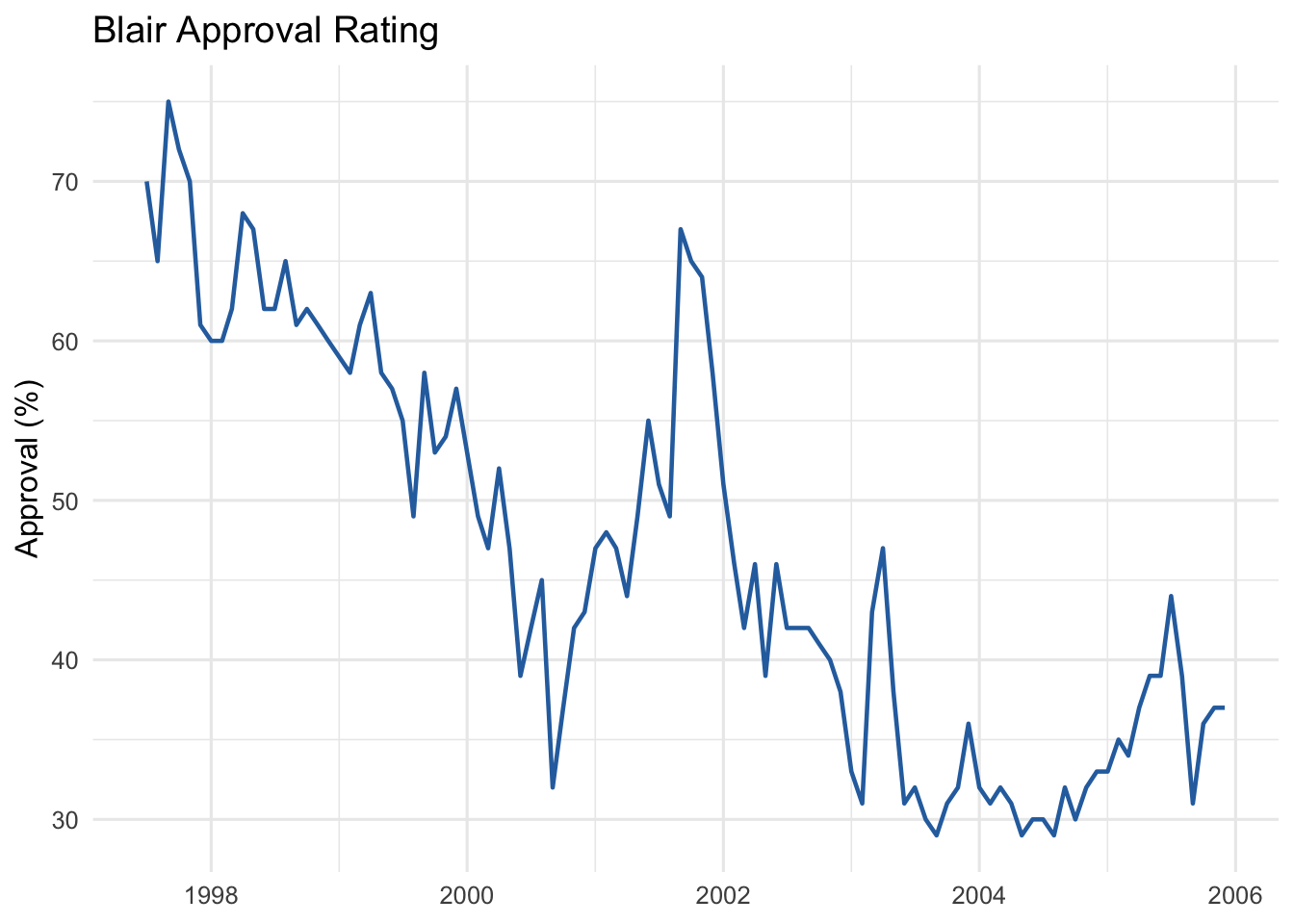
We first plot the approval series to get a sense of its behaviour over time. Visual inspection is always the starting point for time-series analysis — trends and structural breaks often reveal themselves immediately.
The series shows a clear downward trend rather than fluctuating around a constant mean — an early signal that it may be non-stationary (integrated of order 1, or I(1)).
Labour as Best Economic Manager
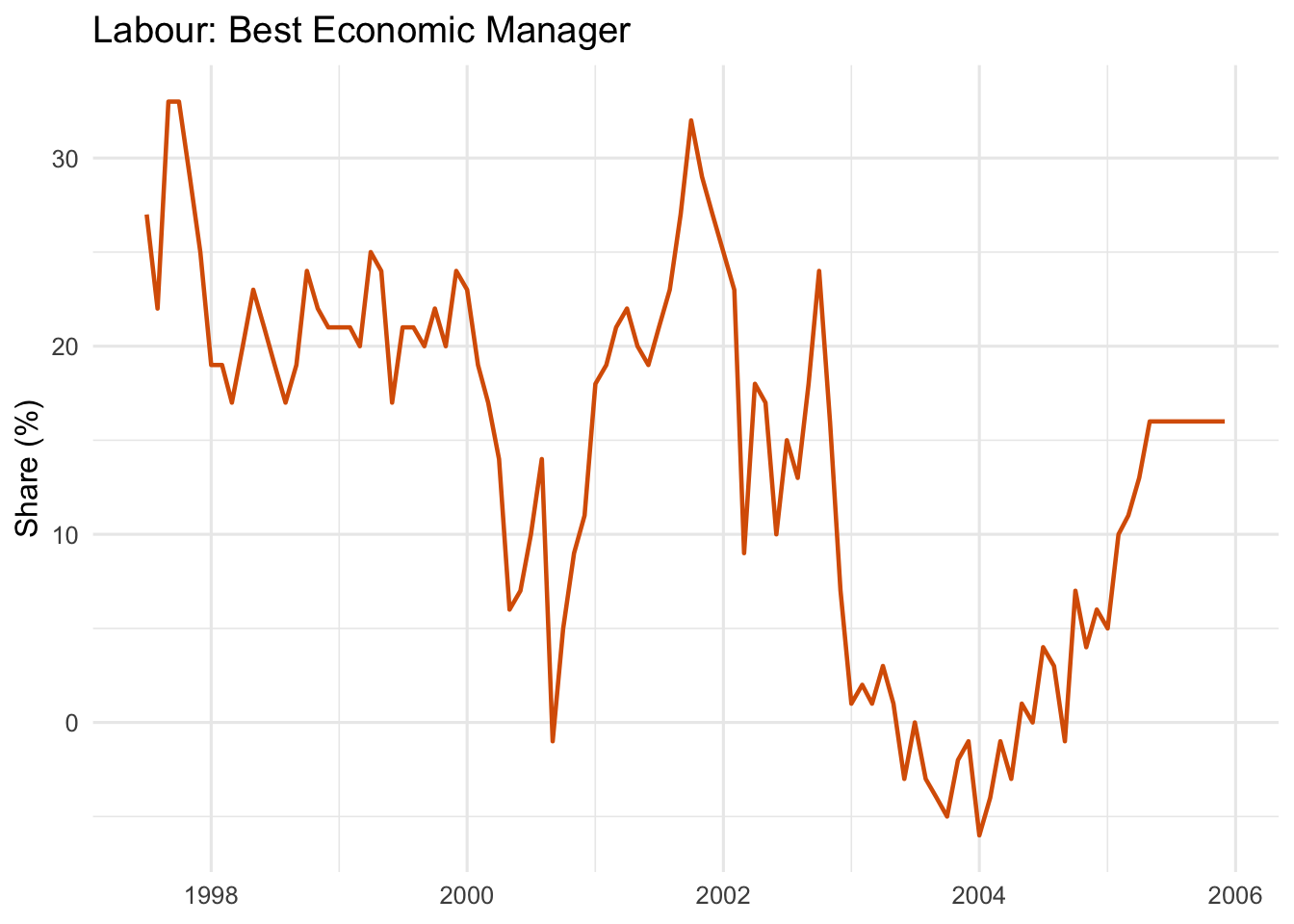
The key independent variable is the share of respondents who identified Labour as the best party to manage the economy (labecman).
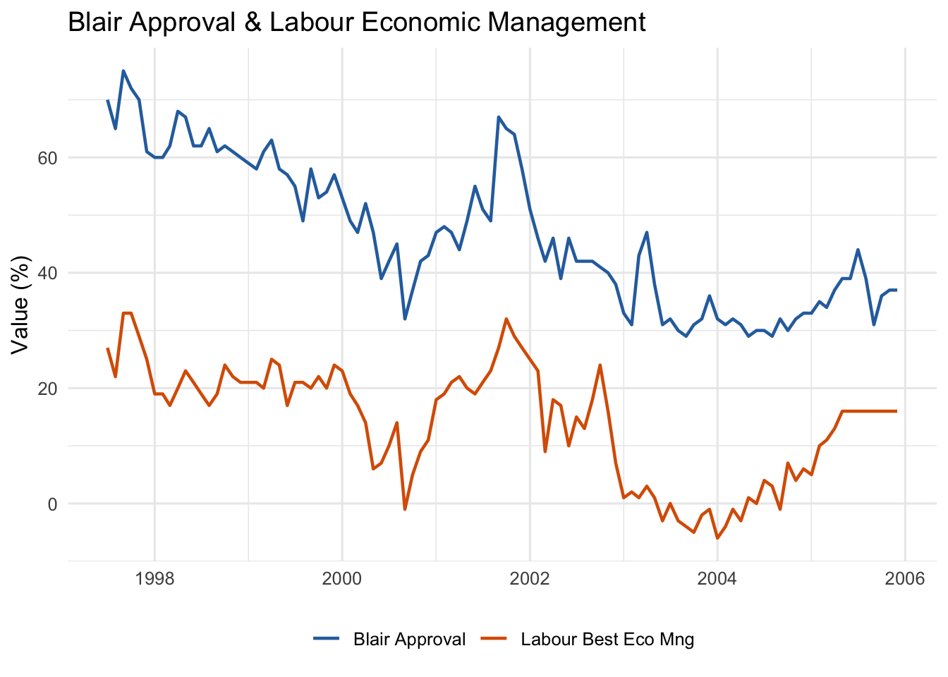
Figure 3: Blair approval and Labour economic management ratings plotted together.
* The || operator overlays a second plot on the same axestwowayline app month || line labecman month
The two series appear to co-move, which motivates both the correlation analysis and the formal cointegration test below.
Correlation
A high pairwise correlation supports the visual impression of co-movement, though it tells us nothing about the direction of causation or whether the relationship is spurious.
# cor.test() returns the correlation coefficient and a two-sided p-value,# equivalent to Stata's pwcorr with the sig option.cor.test(blair$app, blair$labecman)
    Pearson's product-moment correlation

data:  blair$app and blair$labecman
t = 15.007, df = 100, p-value < 2.2e-16
alternative hypothesis: true correlation is not equal to 0
95 percent confidence interval:
 0.7608216 0.8836388
sample estimates:
      cor
0.8321683
* pwcorr displays pairwise correlations; the sig option adds p-values.pwcorr app labecman, sig
Stationarity Testing
Before running any regression, we must establish the order of integration of each series. A series is I(1) (integrated of order 1) if it is non-stationary in levels but becomes stationary after first-differencing.
We use the Augmented Dickey-Fuller (ADF) test throughout.
Null hypothesis: the series has a unit root (is non-stationary).
Reject H₀ (p < 0.05) → the series is stationary.
Fail to reject H₀ → the series is non-stationary; try first differences.
Note on lag selection. Stata’s dfuller defaults to 0 lags with a constant. R’s adf.test() selects lags automatically using \(k = \lfloor (n-1)^{1/3} \rfloor\). Add k = 0 inside adf.test() to replicate Stata’s default exactly.
Warning in adf.test(na.omit(diff(blair$app))): p-value smaller than printed
p-value
    Augmented Dickey-Fuller Test

data:  na.omit(diff(blair$app))
Dickey-Fuller = -5.6329, Lag order = 4, p-value = 0.01
alternative hypothesis: stationary
* Test levels: expect to fail to reject H0 (series is non-stationary)dfuller app* Test first differences: expect to reject H0 (series becomes stationary)* The d. prefix applies the first-difference operatorinlinedfullerd.app
We expect to fail to reject H₀ in levels (the series is I(1)) and reject H₀ in first differences, confirming it becomes stationary after differencing.
Warning in adf.test(na.omit(diff(blair$labecman))): p-value smaller than
printed p-value
    Augmented Dickey-Fuller Test

data:  na.omit(diff(blair$labecman))
Dickey-Fuller = -4.7619, Lag order = 4, p-value = 0.01
alternative hypothesis: stationary
dfuller labecmandfullerd.labecman
If both app and labecman are I(1), the conditions for cointegration are met — we can proceed to the Engle-Granger test.
Cointegration Test (Engle-Granger)
Two I(1) series are cointegrated if there exists a linear combination of them that is I(0) — stationary. Economically, this means they share a long-run equilibrium relationship even though each series individually wanders.
The Engle-Granger (1987) approach tests this in two steps.
Step 1: Estimate the long-run relationship
Regress app on labecman. The fitted line represents the long-run equilibrium. The residuals represent deviations from that equilibrium at each point in time.
coint_reg <-lm(app ~ labecman, data = blair)summary(coint_reg)
Call:
lm(formula = app ~ labecman, data = blair)

Residuals:
     Min       1Q   Median       3Q      Max
-17.6392  -4.7346   0.3458   5.2370  15.2972

Coefficients:
            Estimate Std. Error t value Pr(>|t|)
(Intercept) 31.62244    1.21930   25.93   <2e-16 ***
labecman     1.06355    0.07087   15.01   <2e-16 ***
---
Signif. codes:  0 '***' 0.001 '**' 0.01 '*' 0.05 '.' 0.1 ' ' 1

Residual standard error: 7.038 on 100 degrees of freedom
Multiple R-squared:  0.6925,    Adjusted R-squared:  0.6894
F-statistic: 225.2 on 1 and 100 DF,  p-value: < 2.2e-16
# Save residuals — these become the error correction term in the ECMblair$ecm_labecman <-residuals(coint_reg)
reg app labecman* Save the residuals as a newvariable — this is the error correction termpredict ecm_labecman, resid
Step 2: Test the residuals for stationarity
If the residuals are stationary (I(0)), the series are cointegrated — the deviations from equilibrium are temporary and the series will always revert toward each other. If the residuals are non-stationary, any apparent relationship is spurious.
    Augmented Dickey-Fuller Test

data:  na.omit(blair$ecm_labecman)
Dickey-Fuller = -2.5805, Lag order = 4, p-value = 0.336
alternative hypothesis: stationary
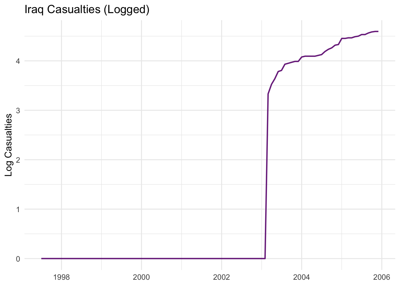
Because casl is non-stationary (it rises monotonically), it enters the ECM as a lagged second-order difference (L2D.casl), which we construct below.
ECM Estimation
Constructing the differenced and lagged variables
The ECM is estimated entirely in first differences (capturing short-run changes), with the lagged residual from the cointegrating regression added as the error correction term. This term tells us: for every 1-unit deviation from the long-run equilibrium last period, how much does the dependent variable adjust this period?
A key difference between R and Stata here is that Stata applies time-series operators inline within the regression command, so no separate variable construction step is needed. In R, we must explicitly create each transformed variable before passing it to lm().
# In Stata, d. / L. / L2D. operators are applied inline at estimation time.# In R, we pre-compute each transformed column explicitly.blair <- blair %>%mutate(d_app =c(NA, diff(app)), # d.appd — dependent variabled_labecman =c(NA, diff(labecman)), # d.labecmanL_ecm_labecman =lag(ecm_labecman, 1), # L.ecm_labecman (error correction term)d_casl =c(NA, diff(casl)), # D.casl (intermediate)L2D_casl =lag(d_casl, 2) # L2D.casl )
* No separatevariable construction is needed in Stata.* The d., L., and L2D. operators are applied directly inside the* regression command. Stata's tsset declaration (made earlier) enables this.* For reference, the operators used in the next step mean:* d.X first difference of X* L.X one-period lag of X* L2D.X two-period lag of the first difference of X* v911d and petrold are already differenced variables in the dataset.
Call:
lm(formula = d_app ~ d_labecman + L_ecm_labecman + v911d + petrold +
    L2D_casl, data = blair)

Residuals:
    Min      1Q  Median      3Q     Max
-9.1334 -2.1822  0.0344  1.7863 12.1770

Coefficients:
               Estimate Std. Error t value Pr(>|t|)
(Intercept)    -0.24650    0.38719  -0.637  0.52592
d_labecman      0.34247    0.10334   3.314  0.00131 **
L_ecm_labecman -0.14981    0.05883  -2.547  0.01252 *
v911d           9.14158    2.72413   3.356  0.00115 **
petrold        -5.62531    2.89994  -1.940  0.05543 .
L2D_casl       -1.95711    1.17158  -1.670  0.09819 .
---
Signif. codes:  0 '***' 0.001 '**' 0.01 '*' 0.05 '.' 0.1 ' ' 1

Residual standard error: 3.811 on 93 degrees of freedom
  (3 observations deleted due to missingness)
Multiple R-squared:  0.3263,    Adjusted R-squared:  0.2901
F-statistic:  9.01 on 5 and 93 DF,  p-value: 5.198e-07
* Stata applies all time-series operators inline.* L.ecm_labecman is the one-period lag of the cointegrating residual —* this is the error correction term.regd.appd d.labecman L.ecm_labecman v911d petrold L2D.casl
Interpreting the results
Term
Interpretation
d_labecman
Short-run effect: a 1-point rise in Labour’s economic ratings this month is associated with a β change in approval this month.
L_ecm_labecman
Error correction speed. Should be negative and significant. A coefficient of, say, −0.3 means 30% of last period’s deviation from equilibrium is corrected each month.
v911d
One-off impact of the September 2001 attacks on approval (already first-differenced).
petrold
One-off impact of the petrol crisis (already first-differenced).
L2D_casl
Effect of rising Iraq casualties, lagged two periods — the media cycle and public opinion formation mean casualties take time to register in polls.
A negative and statistically significantL_ecm_labecman is the crucial result: it confirms that when approval ratings deviate from their long-run relationship with economic perceptions, they adjust back toward equilibrium over subsequent months.
Summary
This analysis followed the standard Engle-Granger ECM procedure:
Visualised the series to identify apparent non-stationarity and co-movement.
Confirmed both series are I(1) via ADF tests on levels and first differences.
Tested for cointegration by regressing app on labecman and confirming that the residuals are I(0).
Estimated the ECM, modelling short-run changes in approval as a function of short-run changes in economic perceptions, the error correction term, and event-based shocks.
The ECM framework is particularly well-suited to approval rating data because it respects the non-stationary nature of the series, recovers the long-run relationship, and separately identifies the speed of adjustment — all of which have substantive political-science meaning.