Multiple Imputation for Cross-Sectional Time Series Data

Implementing Honaker & King (2010) with Amelia II, plm, and Stata mi/xtreg

panel data
code
analysis
Author

Robert W. Walker

Published

July 28, 2026

Background and Motivation

Cross-sectional time series (TSCS) data — also called panel or longitudinal data — pose particular challenges for multiple imputation. Standard imputation methods treat observations as exchangeable, discarding two structural features that TSCS data possess in abundance:

  1. Temporal autocorrelation: an observation for unit \(i\) at time \(t\) is predictable from observations for the same unit at \(t \pm 1, t \pm 2, \ldots\)
  2. Unit-specific trajectories: each cross-sectional unit follows its own trend over time, so a pooled time polynomial is too restrictive.

Honaker and King (2010, AJPS 54:561–581) adapt the EM algorithm to exploit both features. Their software — Amelia II — augments every imputation equation with polynomial functions of time interacted with unit indicators, letting the model borrow information from temporal neighbours within each unit. This recovers much of the information discarded by listwise deletion, which in TSCS settings tends to cluster in time and across units (making the MCAR assumption implausible).

The Missing-Data Taxonomy

Mechanism Condition Consequence for estimators
MCAR \(P(\mathbf{M} \mid \mathbf{Y}) = P(\mathbf{M})\) Listwise deletion is unbiased but inefficient
MAR \(P(\mathbf{M} \mid \mathbf{Y}) = P(\mathbf{M} \mid \mathbf{Y}_\text{obs})\) MI is consistent and efficient
MNAR Depends on unobserved values No off-the-shelf solution; sensitivity analysis required

Honaker and King argue that the MAR assumption is more defensible in TSCS data than it first appears: temporal neighbours of a missing value act as proxies for what was not observed, so the probability of missingness depends primarily on observed quantities.

Rubin’s Combining Rules

Given \(M\) imputed datasets, estimate the quantity of interest \(Q\) in each dataset, obtaining \(\hat{Q}_m\) with estimated variance \(\hat{U}_m\). Rubin (1987) shows valid frequentist inference follows from:

\[\bar{Q} = \frac{1}{M}\sum_{m=1}^{M}\hat{Q}_m\]

\[\bar{U} = \frac{1}{M}\sum_{m=1}^{M}\hat{U}_m \qquad \text{(within-imputation variance)}\]

\[B = \frac{1}{M-1}\sum_{m=1}^{M}(\hat{Q}_m - \bar{Q})^2 \qquad \text{(between-imputation variance)}\]

\[T = \bar{U} + \left(1 + \frac{1}{M}\right)B \qquad \text{(total variance)}\]

The fraction of missing information summarises how much the missing data inflate posterior uncertainty:

\[\hat{\gamma} = \frac{(1 + 1/M)\,B}{T}\]

The Barnard–Rubin (1999) small-sample degrees of freedom are:

\[\nu = (M-1)\!\left[1 + \frac{M\bar{U}}{(M+1)B}\right]^{2}\]

These are what mi estimate in Stata and mi.meld() in R implement.


Data: freetrade

We use the freetrade dataset shipped with the Amelia package. It covers nine Asian countries over 1980–1999 and was assembled to study the determinants of trade liberalisation. The dependent variable of interest is tariff (average tariff rate in percent), and key covariates are:

Variable Description Scale
tariff Average tariff rate (%) Continuous
polity Democracy score (Polity IV) −10 to +10
pop Population Continuous (right-skewed)
gdp.pc GDP per capita Continuous (right-skewed)
intresmi Real interest rate Continuous
signed IMF agreement signed Binary
fiveop Five-year trade openness Continuous
usheg US trade hegemony Continuous

The dataset is also available as the Stata example dataset webuse freetrade, enabling exact replication across platforms.

data("freetrade", package = "Amelia")
glimpse(freetrade)
Rows: 171
Columns: 10
$ year     <int> 1981, 1982, 1983, 1984, 1985, 1986, 1987, 1988, 1989, 1990, 1…
$ country  <chr> "SriLanka", "SriLanka", "SriLanka", "SriLanka", "SriLanka", "…
$ tariff   <dbl> NA, NA, 41.3, NA, 31.0, NA, 27.3, 27.3, NA, 28.3, 26.9, 25.0,…
$ polity   <int> 6, 5, 5, 5, 5, 5, 5, 5, 5, 5, 5, 5, 5, 5, 5, 5, 5, 5, 6, 8, 8…
$ pop      <dbl> 14988000, 15189000, 15417000, 15599000, 15837000, 16117000, 1…
$ gdp.pc   <dbl> 461.0236, 473.7634, 489.2266, 508.1739, 525.5609, 538.9237, 5…
$ intresmi <dbl> 1.937347, 1.964430, 1.663936, 2.797462, 2.259116, 1.832549, 1…
$ signed   <int> 0, 0, 1, 0, 0, 0, 0, 1, 0, 0, 1, NA, 0, 0, 0, 0, 0, 0, 0, 1, …
$ fiveop   <dbl> 12.4, 12.5, 12.3, 12.3, 12.3, 12.5, 12.5, 12.6, 12.6, 12.7, 1…
$ usheg    <dbl> 0.2593112, 0.2558008, 0.2655022, 0.2988009, 0.2952431, 0.2886…
* freetrade ships as a Stata example dataset — no installation needed
webuse freetrade, clear
describe
label list   // country labels if stored as value-labelled numeric

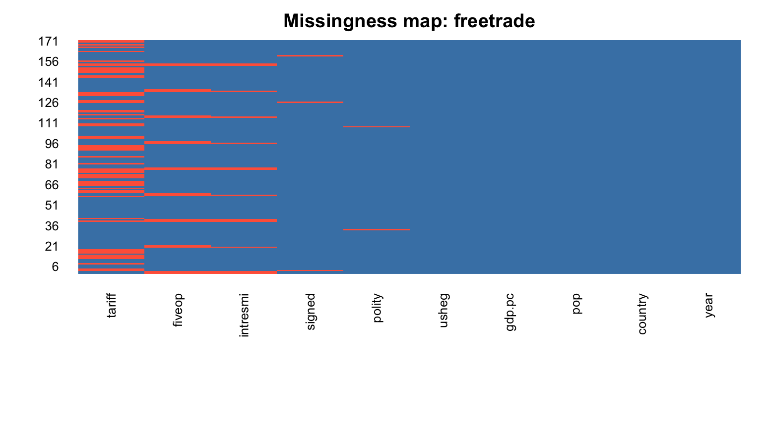
Missingness Patterns

# Classic Amelia missingness map
missmap(freetrade,
        main   = "Missingness map: freetrade",
        col    = c("tomato", "steelblue"),
        legend = FALSE,
        margins = c(8, 4))

miss_var_summary(freetrade) |>
  filter(n_miss > 0) |>
  gt() |>
  tab_header(title = "Missing data summary") |>
  fmt_number(columns = pct_miss, decimals = 1) |>
  cols_label(variable = "Variable", n_miss = "N missing", pct_miss = "% missing")
Missing data summary
Variable N missing % missing
tariff 58 33.9
fiveop 18 10.5
intresmi 13 7.60
signed 3 1.75
polity 2 1.17
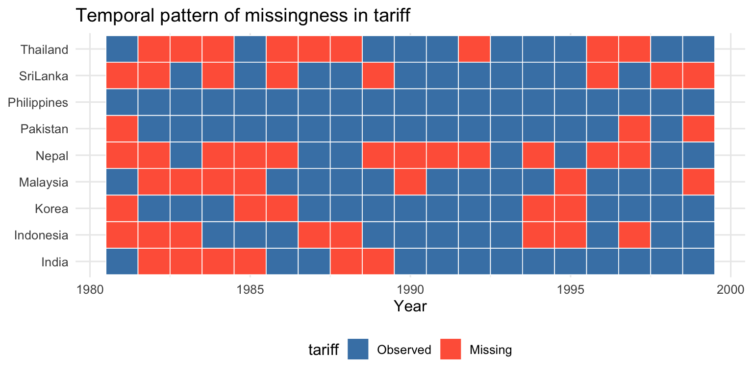
# Missingness over time for tariff by country
freetrade |>
  mutate(tariff_missing = is.na(tariff)) |>
  ggplot(aes(x = year, y = country, fill = tariff_missing)) +
  geom_tile(colour = "white", linewidth = 0.3) +
  scale_fill_manual(values = c("steelblue", "tomato"),
                    labels = c("Observed", "Missing"),
                    name   = "tariff") +
  labs(title = "Temporal pattern of missingness in tariff",
       x = "Year", y = NULL) +
  theme_minimal(base_size = 12) +
  theme(legend.position = "bottom")

* Summary of missing values
misstable summarize tariff polity intresmi
misstable patterns tariff polity intresmi, frequency

* Visualise missingness over time for tariff (requires tabplot from SSC)
* ssc install tabplot, replace
tabplot country year if missing(tariff), ///
    title("Missing tariff by country and year") scheme(s2color)

Imputation with Amelia

Amelia fits an expectation-maximisation with importance sampling (EMis) model under the assumption of approximate multivariate normality. For TSCS data, Honaker and King (2010) recommend the following additional options:

Argument Purpose
ts = "year" Identifies the time variable
cs = "country" Identifies the cross-sectional unit
polytime = 2 Adds quadratic polynomial in time to each imputation equation
intercs = TRUE Interacts the time polynomial with unit dummies (unit-specific trends)
lags = "tariff" Adds \(\text{tariff}_{t-1}\) as a predictor (AR structure)
leads = "tariff" Adds \(\text{tariff}_{t+1}\) as a predictor (forward-looking borrowing)
logs = c("pop","gdp.pc") Log-transforms right-skewed variables before imputation

The combination of polytime and intercs = TRUE is the key innovation: it means each country gets its own quadratic time trend in every imputation equation, so a missing tariff for Thailand in 1992 is informed primarily by Thailand’s own trajectory rather than a cross-country average.

set.seed(20240601)

a.out <- amelia(
  x        = freetrade,
  m        = 20,              # 20 imputations; ≈ % missing is a useful heuristic
  ts       = "year",
  cs       = "country",
  polytime = 2,               # quadratic within-unit time trend
  intercs  = TRUE,            # unit × trend interactions (key Honaker-King innovation)
  lags     = "tariff",        # AR(1) borrowing
  leads    = "tariff",        # forward borrowing
  logs     = c("pop", "gdp.pc"),  # log-transform before EMis
  p2s      = 0                # suppress iteration-by-iteration output
)

summary(a.out)

Amelia output with 20 imputed datasets.
Return code:  1 
Message:  Normal EM convergence. 

Chain Lengths:
--------------
Imputation 1:  467
Imputation 2:  1266
Imputation 3:  374
Imputation 4:  531
Imputation 5:  298
Imputation 6:  162
Imputation 7:  328
Imputation 8:  426
Imputation 9:  2707
Imputation 10:  1187
Imputation 11:  426
Imputation 12:  3644
Imputation 13:  247
Imputation 14:  706
Imputation 15:  1237
Imputation 16:  734
Imputation 17:  407
Imputation 18:  332
Imputation 19:  1471
Imputation 20:  405

Rows after Listwise Deletion:  96 
Rows after Imputation:  171 
Patterns of missingness in the data:  8 

Fraction Missing for original variables: 
-----------------------------------------

         Fraction Missing
year           0.00000000
country        0.00000000
tariff         0.33918129
polity         0.01169591
pop            0.00000000
gdp.pc         0.00000000
intresmi       0.07602339
signed         0.01754386
fiveop         0.10526316
usheg          0.00000000
* ── Prepare data ────────────────────────────────────────────────────────────
encode country, gen(cid)         // mi requires numeric cross-section id
xtset cid year

* Log-transform skewed covariates
gen lpop   = log(pop)
gen lgdppc = log(gdppc)          // NB: Stata's webuse spells this gdppc

* ── Approximate Honaker-King TSCS structure ─────────────────────────────────
* Create within-unit polynomial time trends (≈ polytime=2, intercs=TRUE)
bysort cid (year): gen t_trend  = _n
gen t_trend2 = t_trend ^ 2

* Lags and leads for AR structure (≈ lags="tariff", leads="tariff")
bysort cid (year): gen L1_tariff = tariff[_n - 1]
bysort cid (year): gen F1_tariff = tariff[_n + 1]

* ── Declare MI structure and impute ─────────────────────────────────────────
mi set mlong

* Multivariate normal imputation (EMis) — closest Stata equivalent to Amelia
mi impute mvn tariff polity intresmi =                  ///
    lpop lgdppc signed fiveop usheg                     ///  substantive vars
    i.cid c.t_trend##c.t_trend                          ///  unit-specific trends
    L1_tariff F1_tariff,                                ///  temporal borrowing
    add(20) rseed(20240601) iterate(500)

mi describe

* Note: Stata's mi impute chained is also possible and may handle
* non-normal variables better, but requires specifying each variable's
* imputation model separately.

Imputation Diagnostics

Good imputation practice requires checking that imputed values are plausible. Honaker and King (2010) suggest two primary diagnostics.

Density overlap

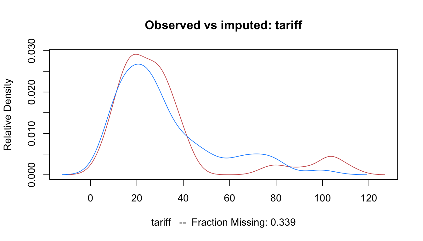
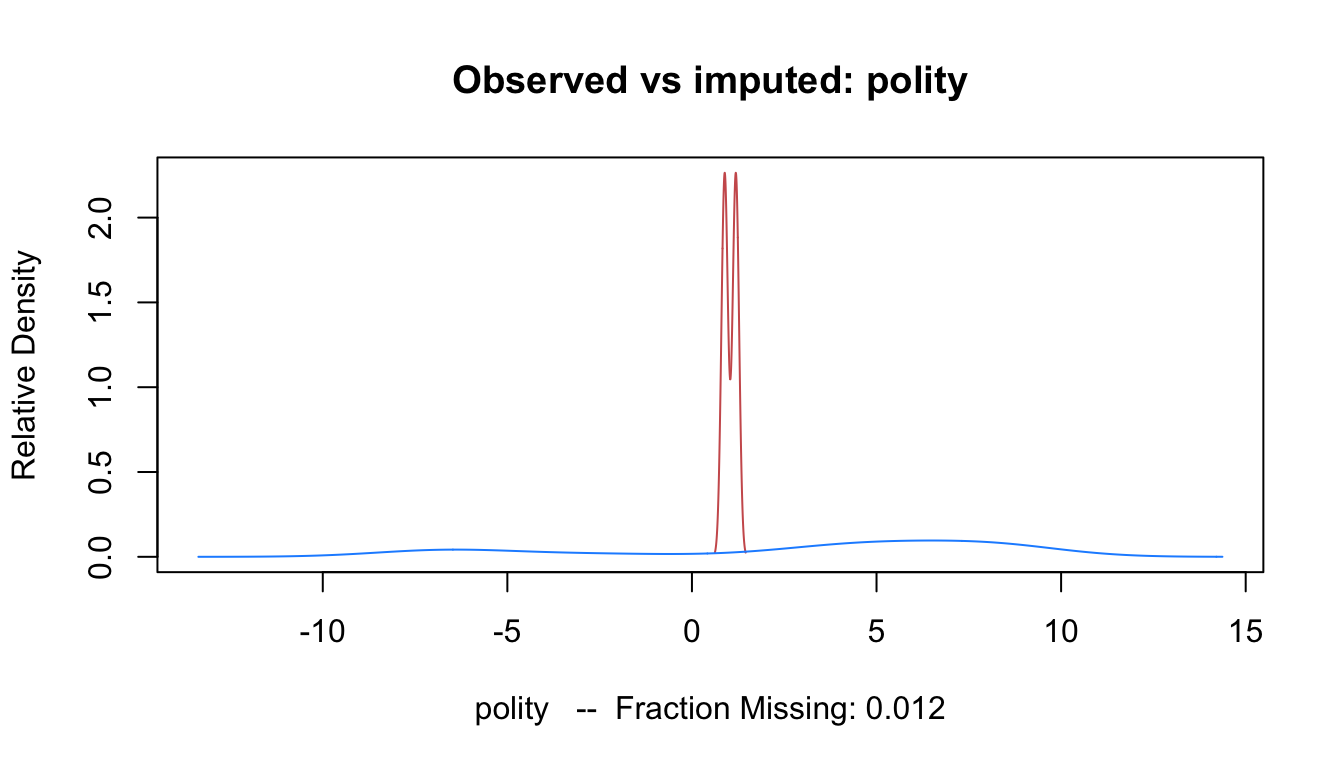
Imputed values (red) should be broadly consistent with observed values (black): the same support and rough shape. Systematic divergence suggests model misspecification.

plot(a.out, which.vars = "tariff",
     main = "Observed vs imputed: tariff")

plot(a.out, which.vars = "polity",
     main = "Observed vs imputed: polity")

* Overlay kernel densities of observed vs imputed tariff across imputations
mi convert wide, clear

* Use twoway plot over all m datasets
local cmd ""
forvalues m = 1/20 {
    local cmd `cmd' (kdensity tariff_`m', lcolor(red%30) lwidth(thin))
}
twoway (kdensity tariff, lcolor(black) lwidth(medium) lpattern(solid)) ///
    `cmd', ///
    legend(order(1 "Observed" 2 "Imputed (m=1..20)")) ///
    title("Density: observed vs imputed tariff") xtitle("Tariff rate")

mi convert mlong, clear   // restore long format

Over-imputation (model checking)

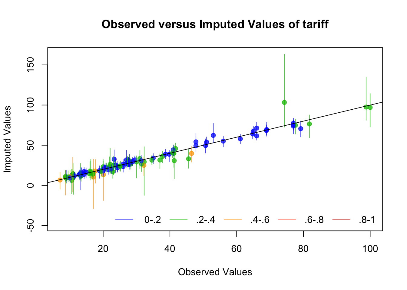
Artificially set observed values to missing, re-impute them, and check that the 90% imputation intervals cover the true observed values at the expected rate (~90%). A systematic over- or under-coverage pattern reveals model misspecification.

overimpute(a.out, var = "tariff")

* Over-imputation is not available in Stata's native mi suite.
*
* Recommended workflow: impute in R with Amelia, run overimpute() there
* for diagnostics, then export to Stata for analysis:
*
*   # In R:
*   overimpute(a.out, var = "tariff")           # check model
*   write.amelia(a.out, file.stem = "ft_imp",   # export
*                format = "dta")
*
* See Section 7 for the full export/import workflow.

Panel Data Analysis

We now pool across imputations using Rubin’s combining rules. The model is a standard panel specification:

\[\text{tariff}_{it} = \alpha_i + \beta_1\,\text{polity}_{it} + \beta_2\,\ln(\text{pop}_{it}) + \beta_3\,\ln(\text{gdp.pc}_{it}) + \varepsilon_{it}\]

where \(\alpha_i\) are country fixed effects (absorbed by the within transformation in the FE estimator, or modelled as random draws in the RE estimator).

Pooling helper function

The key function pools plm estimates across imputations using mi.meld() from Amelia and appends the Barnard–Rubin degrees of freedom and fraction of missing information for each coefficient.

#' Pool plm estimates across Amelia imputations (Rubin's combining rules)
#'
#' @param amelia_out  An object of class 'amelia' (output of amelia())
#' @param formula     Model formula passed to plm()
#' @param index       Panel index, e.g. c("country", "year")
#' @param model       "within" (FE) or "random" (RE)
#' @param ...         Additional arguments passed to plm()
#' @return A tibble with pooled estimates, Rubin SE, B-R df, and FMI
pool_plm <- function(amelia_out, formula, index, model, ...) {

  # 1. Fit plm to each imputed dataset
  fits <- lapply(amelia_out$imputations, function(d) {
    plm(formula, data = d, index = index, model = model, ...)
  })

  # 2. Extract Q̂ (M × K) and SE (M × K)
  Q  <- do.call(rbind, lapply(fits, coef))
  SE <- do.call(rbind, lapply(fits, function(f) sqrt(diag(vcov(f)))))

  # 3. Rubin's combining rules via mi.meld()
  pooled <- mi.meld(q = Q, se = SE)          # returns 1×K matrices
  est    <- as.numeric(pooled$q.mi)
  se_mi  <- as.numeric(pooled$se.mi)

  # 4. Barnard-Rubin (1999) degrees of freedom
  M    <- nrow(Q)
  Ubar <- colMeans(SE^2)                     # within-imputation variance
  B    <- apply(Q, 2, var)                   # between-imputation variance
  T_   <- Ubar + (1 + 1/M) * B              # total variance
  gamma <- (1 + 1/M) * B / T_               # fraction of missing information
  df_BR <- (M - 1) * (1 + Ubar / ((1 + 1/M) * B))^2

  # 5. Assemble tidy tibble
  tibble(
    term      = colnames(Q),
    estimate  = est,
    std.error = se_mi,
    statistic = est / se_mi,
    df        = df_BR,
    p.value   = 2 * pt(-abs(est / se_mi), df = df_BR),
    fmi       = gamma,
    W_var     = Ubar,
    B_var     = B,
    T_var     = T_
  )
}
* In Stata, mi estimate pools automatically — no helper function needed.
* It implements Rubin's combining rules and the Barnard-Rubin df adjustment.
*
* mi estimate stores the between- and within-imputation variance matrices:
*   e(V_Ubar)  — within-imputation covariance matrix
*   e(V_B)     — between-imputation covariance matrix
*   e(V_Q)     — total (Rubin) covariance matrix
*   e(fmi)     — fraction of missing information (vector)

Fixed-Effects Model

The within estimator removes all time-invariant confounding. Under FE, the coefficient on polity identifies the effect of within-country changes in democracy on tariff rates.

panel_formula <- tariff ~ polity + log(pop) + log(gdp.pc)

res_fe <- pool_plm(
  amelia_out = a.out,
  formula    = panel_formula,
  index      = c("country", "year"),
  model      = "within"
)

res_fe |>
  select(term, estimate, std.error, statistic, df, p.value, fmi) |>
  gt() |>
  tab_header(
    title    = "Fixed-Effects Model — MI Pooled (M = 20)",
    subtitle = "Dependent variable: tariff rate (%)"
  ) |>
  fmt_number(columns = c(estimate, std.error, statistic, p.value, fmi),
             decimals = 4) |>
  fmt_number(columns = df, decimals = 1) |>
  cols_label(
    term      = "Coefficient",
    estimate  = "Q̄",
    std.error = "SE (Rubin)",
    statistic = "t",
    df        = "df (B–R)",
    p.value   = "p",
    fmi       = "FMI"
  ) |>
  tab_style(
    style     = cell_fill(color = "#fef9c3"),
    locations = cells_body(rows = p.value < 0.05)
  )
Fixed-Effects Model — MI Pooled (M = 20)
Dependent variable: tariff rate (%)
Coefficient SE (Rubin) t df (B–R) p FMI
polity 0.1300 0.3453 0.3765 100.4 0.7074 0.4350
log(pop) −58.6025 19.7489 −2.9674 56.5 0.0044 0.5800
log(gdp.pc) −9.0373 7.7276 −1.1695 101.2 0.2450 0.4334
* ── Fixed effects ────────────────────────────────────────────────────────────
mi estimate, dots notable: xtreg tariff polity lpop lgdppc, fe

* The notable option prints the between- and within-variance components.
* mi estimate output includes:
*   - Pooled estimates (Q̄)
*   - Rubin standard errors (√T)
*   - Barnard-Rubin degrees of freedom
*   - Fraction of missing information per coefficient
*   - Relative efficiency = 1 / (1 + FMI/M)

* Store for later comparison
estimates store mi_fe

Random-Effects Model

The GLS random-effects estimator assumes \(\alpha_i \perp \mathbf{X}_{it}\). It is more efficient than FE when this assumption holds, because it exploits between-unit variation as well as within-unit variation.

res_re <- pool_plm(
  amelia_out = a.out,
  formula    = panel_formula,
  index      = c("country", "year"),
  model      = "random"
)

res_re |>
  select(term, estimate, std.error, statistic, df, p.value, fmi) |>
  gt() |>
  tab_header(
    title    = "Random-Effects Model — MI Pooled (M = 20)",
    subtitle = "Dependent variable: tariff rate (%)"
  ) |>
  fmt_number(columns = c(estimate, std.error, statistic, p.value, fmi),
             decimals = 4) |>
  fmt_number(columns = df, decimals = 1) |>
  cols_label(
    term      = "Coefficient",
    estimate  = "Q̄",
    std.error = "SE (Rubin)",
    statistic = "t",
    df        = "df (B–R)",
    p.value   = "p",
    fmi       = "FMI"
  ) |>
  tab_style(
    style     = cell_fill(color = "#fef9c3"),
    locations = cells_body(rows = p.value < 0.05)
  )
Random-Effects Model — MI Pooled (M = 20)
Dependent variable: tariff rate (%)
Coefficient SE (Rubin) t df (B–R) p FMI
(Intercept) 113.2657 98.8233 1.1461 54.3 0.2568 0.5914
polity −0.4506 0.2833 −1.5904 391.3 0.1125 0.2204
log(pop) 1.7602 4.8798 0.3607 64.5 0.7195 0.5429
log(gdp.pc) −16.3099 3.6172 −4.5090 138.0 0.0000 0.3710
* ── Random effects ───────────────────────────────────────────────────────────
mi estimate, dots notable: xtreg tariff polity lpop lgdppc, re
estimates store mi_re

Complete-Case Comparison

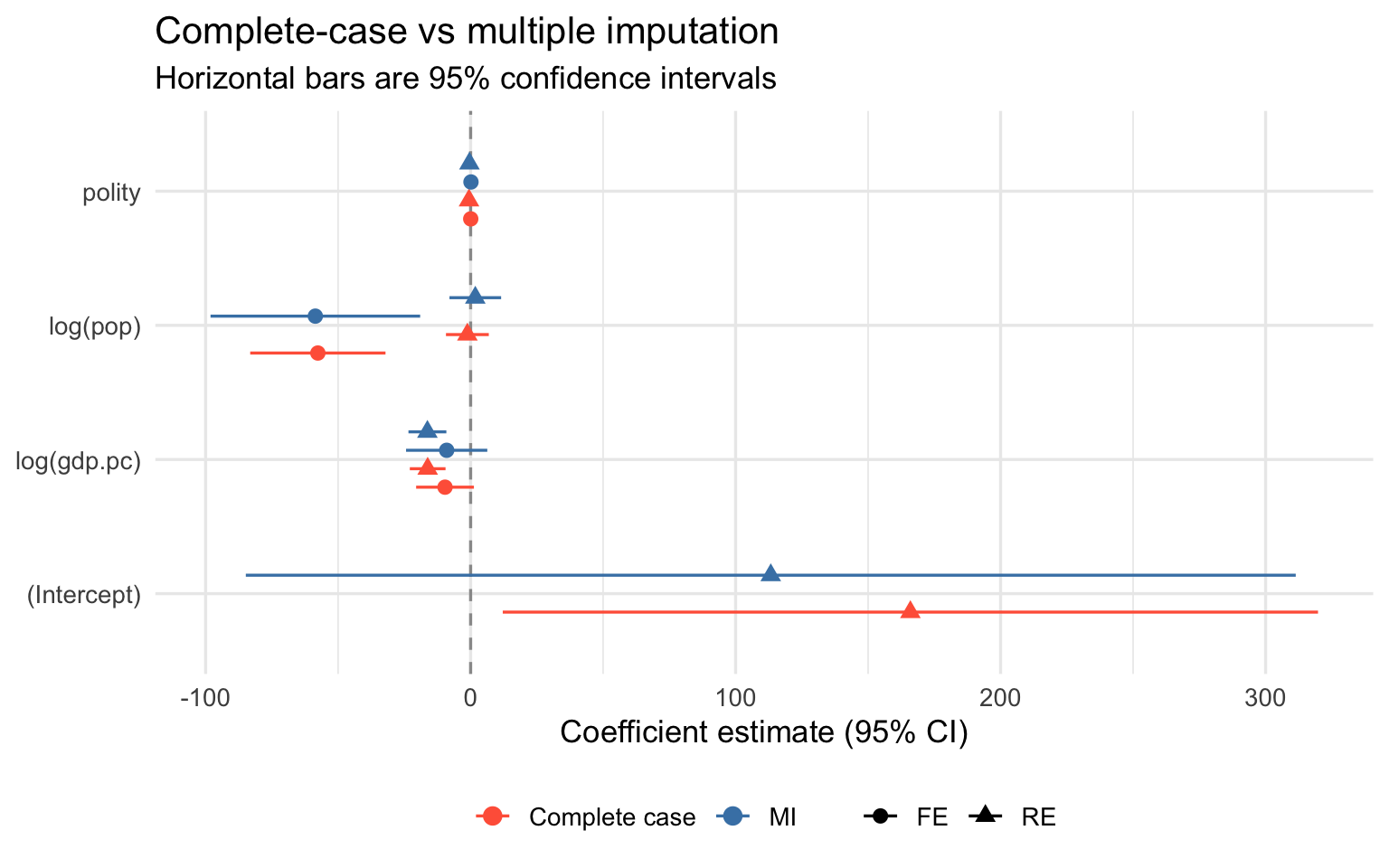
How much does listwise deletion distort our estimates? We fit the same FE and RE models on the complete cases and plot all four sets of estimates side-by-side.

# Complete-case models on the raw data
cc_fe_tidy <- plm(panel_formula, data = freetrade,
                  index = c("country", "year"), model = "within") |>
  tidy(conf.int = TRUE) |>
  mutate(method = "Complete case – FE")

cc_re_tidy <- plm(panel_formula, data = freetrade,
                  index = c("country", "year"), model = "random") |>
  tidy(conf.int = TRUE) |>
  mutate(method = "Complete case – RE")

# Tidy MI results — use z ≈ 1.96 for wide CIs; exact via qt(0.975, df)
mi_fe_tidy <- res_fe |>
  mutate(
    conf.low  = estimate - qt(0.975, df) * std.error,
    conf.high = estimate + qt(0.975, df) * std.error,
    method    = "MI (Amelia) – FE"
  )

mi_re_tidy <- res_re |>
  mutate(
    conf.low  = estimate - qt(0.975, df) * std.error,
    conf.high = estimate + qt(0.975, df) * std.error,
    method    = "MI (Amelia) – RE"
  )

# Stack for plotting
plot_df <- bind_rows(
  cc_fe_tidy |> select(term, estimate, conf.low, conf.high, method),
  cc_re_tidy |> select(term, estimate, conf.low, conf.high, method),
  mi_fe_tidy |> select(term, estimate, conf.low, conf.high, method),
  mi_re_tidy |> select(term, estimate, conf.low, conf.high, method)
) |>
  mutate(
    estimator = if_else(str_detect(method, "FE"), "FE", "RE"),
    imputed   = if_else(str_detect(method, "MI"), "MI", "Complete case")
  )

ggplot(plot_df,
       aes(x = estimate, y = term,
           colour = imputed, shape = estimator,
           xmin = conf.low, xmax = conf.high)) +
  geom_vline(xintercept = 0, linetype = "dashed", colour = "grey60") +
  geom_pointrange(position = position_dodge(width = 0.55), size = 0.55) +
  scale_colour_manual(values = c("Complete case" = "tomato",
                                 "MI"            = "steelblue"),
                      name = NULL) +
  scale_shape_manual(values = c("FE" = 16, "RE" = 17), name = NULL) +
  labs(
    x       = "Coefficient estimate (95% CI)",
    y       = NULL,
    title   = "Complete-case vs multiple imputation",
    subtitle = "Horizontal bars are 95% confidence intervals"
  ) +
  theme_minimal(base_size = 13) +
  theme(legend.position = "bottom")

* ── Complete-case ────────────────────────────────────────────────────────────
xtreg tariff polity lpop lgdppc, fe
estimates store cc_fe

xtreg tariff polity lpop lgdppc, re
estimates store cc_re

* ── Coefficient table ────────────────────────────────────────────────────────
esttab cc_fe cc_re mi_fe mi_re,                              ///
    b(4) se(4) star(* 0.10 ** 0.05 *** 0.01)                 ///
    title("Complete-case vs MI estimates: tariff")            ///
    mtitles("CC–FE" "CC–RE" "MI–FE" "MI–RE")                 ///
    note("Rubin SE for MI models. Barnard-Rubin df.")

* ── Coefficient plot (requires coefplot, ssc install coefplot) ───────────────
coefplot (cc_fe, label("Complete case FE") msymbol(O) mcolor(tomato))  ///
         (mi_fe, label("MI FE")            msymbol(D) mcolor(navy)),    ///
    drop(_cons) xline(0) bycoefs                                         ///
    title("Complete-case vs MI: Fixed effects") legend(rows(1))

Variance Decomposition and Missing-Information Diagnostics

Rubin’s Between–Within Decomposition

The between-imputation variance \(B\) and within-imputation variance \(\bar{U}\) tell us qualitatively different things:

  • Large \(\bar{U}\) with small \(B\): the sample itself is small or noisy; more data would help more than better imputation.
  • Large \(B\) with small \(\bar{U}\): the coefficient is well-estimated in each imputed dataset, but the imputed values vary a lot across datasets — the missing data are doing heavy lifting.
bw_table <- bind_rows(
  res_fe |> mutate(model = "Fixed Effects"),
  res_re |> mutate(model = "Random Effects")
) |>
  select(model, term, W_var, B_var, T_var, fmi) |>
  mutate(
    pct_between = round(100 * B_var / T_var, 1),
    across(c(W_var, B_var, T_var), ~ round(.x, 6)),
    fmi = round(fmi, 4)
  )

bw_table |>
  gt(groupname_col = "model") |>
  tab_header(
    title    = "Between–Within Variance Decomposition (Rubin)",
    subtitle = "M = 20 imputations"
  ) |>
  cols_label(
    term        = "Coefficient",
    W_var       = "Within (Ū)",
    B_var       = "Between (B)",
    T_var       = "Total (T)",
    fmi         = "FMI",
    pct_between = "% due to MI"
  ) |>
  tab_footnote(
    footnote  = "FMI: fraction of missing information = (1 + 1/M)B / T",
    locations = cells_column_labels(columns = fmi)
  )
Between–Within Variance Decomposition (Rubin)
M = 20 imputations
Coefficient Within (Ū) Between (B) Total (T) FMI1 % due to MI
Fixed Effects
polity 0.067380 0.049404 0.119254 0.4350 41.4
log(pop) 163.795326 215.452556 390.020510 0.5800 55.2
log(gdp.pc) 33.836351 24.647593 59.716323 0.4334 41.3
Random Effects
(Intercept) 3990.549246 5500.476014 9766.049061 0.5914 56.3
polity 0.062595 0.016849 0.080286 0.2204 21.0
log(pop) 10.885247 12.311789 23.812626 0.5429 51.7
log(gdp.pc) 8.229371 4.623550 13.084099 0.3710 35.3
1 FMI: fraction of missing information = (1 + 1/M)B / T
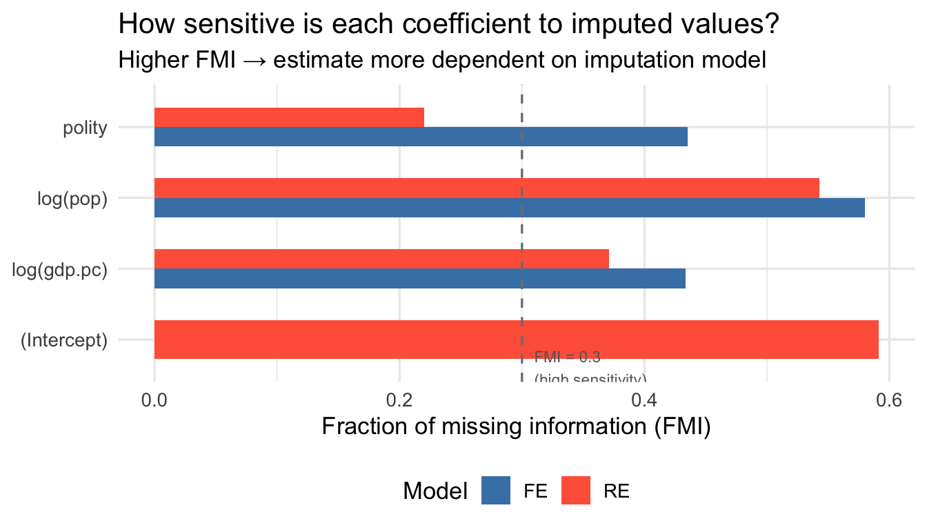
bind_rows(
  res_fe |> mutate(model = "FE"),
  res_re |> mutate(model = "RE")
) |>
  ggplot(aes(x = fmi, y = term, fill = model)) +
  geom_col(position = "dodge", width = 0.55) +
  geom_vline(xintercept = 0.3, linetype = "dashed", colour = "grey50") +
  scale_fill_manual(values = c("FE" = "steelblue", "RE" = "tomato"),
                    name = "Model") +
  annotate("text", x = 0.31, y = 0.6, label = "FMI = 0.3\n(high sensitivity)",
           hjust = 0, size = 3, colour = "grey40") +
  labs(
    x       = "Fraction of missing information (FMI)",
    y       = NULL,
    title   = "How sensitive is each coefficient to imputed values?",
    subtitle = "Higher FMI → estimate more dependent on imputation model"
  ) +
  theme_minimal(base_size = 13) +
  theme(legend.position = "bottom")

* ── Retrieve stored variance matrices after mi estimate ──────────────────────
mi estimate, dots: xtreg tariff polity lpop lgdppc, fe

matrix W  = e(V_Ubar)     // within-imputation covariance
matrix B  = e(V_B)        // between-imputation covariance
matrix T  = e(V_Q)        // total (Rubin) covariance
matrix fmi = e(fmi)       // vector of FMI values

matrix list W
matrix list B
matrix list fmi

* Fraction due to between-imputation variance for each coefficient:
* pct_between = diag(B) ./ diag(T) * 100   (element-wise)
local M = 20
matrix adj_B = (`M' + 1) / `M' * B    // (1 + 1/M)*B
* Compare to diag(T) = diag(W) + diag(adj_B)

FE vs RE: The Hausman Test under Multiple Imputation

The standard Hausman test is a quadratic form in the difference \(\hat{\beta}_{FE} - \hat{\beta}_{RE}\) and does not pool straightforwardly under Rubin’s rules. Two tractable alternatives exist.

Option A: Per-Imputation Hausman Tests

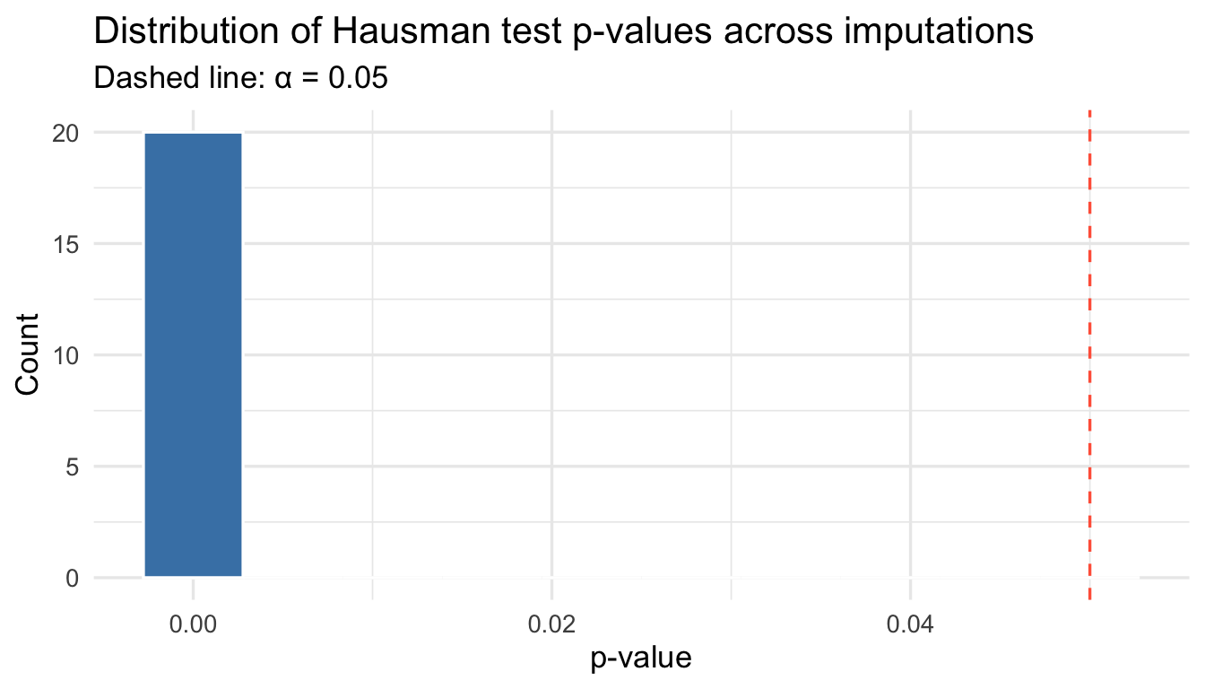
Run the Hausman test in each of the \(M\) imputed datasets and inspect the distribution of \(\chi^2\) statistics or \(p\)-values.

haus_stats <- lapply(seq_along(a.out$imputations), function(m) {
  d  <- a.out$imputations[[m]]
  fe <- plm(panel_formula, data = d, index = c("country", "year"), model = "within")
  re <- plm(panel_formula, data = d, index = c("country", "year"), model = "random")
  ht <- phtest(fe, re)
  tibble(m = m, statistic = ht$statistic, p.value = ht$p.value, df = ht$parameter)
})

haus_df <- bind_rows(haus_stats)

haus_df |>
  summarise(
    mean_chi2 = round(mean(statistic), 3),
    sd_chi2   = round(sd(statistic), 3),
    pct_reject = round(mean(p.value < 0.05) * 100, 1)
  ) |>
  gt() |>
  tab_header(title = "Hausman test across M = 20 imputations",
             subtitle = "H₀: RE consistent (random effects ≡ fixed effects)") |>
  cols_label(mean_chi2  = "Mean χ²",
             sd_chi2    = "SD χ²",
             pct_reject = "% reject at α=0.05")
Hausman test across M = 20 imputations
H₀: RE consistent (random effects ≡ fixed effects)
Mean χ² SD χ² % reject at α=0.05
64.583 40.098 100
ggplot(haus_df, aes(x = p.value)) +
  geom_histogram(bins = 10, fill = "steelblue", colour = "white") +
  geom_vline(xintercept = 0.05, linetype = "dashed", colour = "tomato") +
  labs(
    x       = "p-value",
    y       = "Count",
    title   = "Distribution of Hausman test p-values across imputations",
    subtitle = "Dashed line: α = 0.05"
  ) +
  theme_minimal(base_size = 13)

* ── Hausman across imputations ────────────────────────────────────────────────
* Store FE and RE in each imputed dataset and run hausman
local reject = 0
forvalues m = 1/20 {
    quietly xtreg tariff polity lpop lgdppc if _mi_m == `m', fe
    estimates store fe_`m'
    quietly xtreg tariff polity lpop lgdppc if _mi_m == `m', re
    estimates store re_`m'
    quietly hausman fe_`m' re_`m'
    if r(p) < 0.05 local reject = `reject' + 1
    display "m=`m': chi2=" r(chi2) "  p=" r(p)
}
display "Rejections at 5%: `reject' / 20"

Exporting Amelia Imputations to Stata

If you prefer to impute in R (for the TSCS-specific features) and analyse in Stata, write.amelia() exports all imputed datasets as .dta files.

# Export: creates freetrade_imp0.dta (original) and
#         freetrade_imp1.dta … freetrade_imp20.dta
write.amelia(a.out,
             file.stem     = "freetrade_imp",
             format        = "dta",
             original.data = TRUE)
* ── Import Amelia imputations into Stata's mi framework ──────────────────────
* (run after write.amelia() in R)

* Option A — manual long stack then mi import
clear
forvalues m = 0/20 {
    append using freetrade_imp`m'.dta
    replace _mi_m = `m' if _mi_m == .   // tag imputation number
}
* Declare as flong (stacked) MI data
mi import flong, m(_mi_m) id(country year)

* Recode string country to numeric if needed
encode country, gen(cid)
mi xtset cid year

* ── Replicate FE and RE from R ───────────────────────────────────────────────
gen lpop   = log(pop)
gen lgdppc = log(gdppc)

mi estimate, dots: xtreg tariff polity lpop lgdppc, fe
mi estimate, dots: xtreg tariff polity lpop lgdppc, re

* ── Option B — use mi import directly (Stata 14+) ────────────────────────────
* If write.amelia() outputs a numbered series, mi import can read them:
* mi import flong using freetrade_imp, m(1/20) id(country year) clear