Day 10.1: Causal Inference in Panels and TWFE

panel data
code
analysis
Author

Robert W. Walker

Published

August 1, 2026

Topic: Staggered treatment timing, two-way fixed effects (TWFE), and modern robust estimators Reference Data: mpdta (Callaway–Sant’Anna 2021; also used in Goodman-Bacon 2021 and Sun–Abraham 2021) Date: July 2026


There is a very useful guide for practitioners.

1. The Setting: Staggered Adoption

In staggered adoption, units become treated at different calendar times \(g \in \{2, \dots, T\}\). A unit \(i\) in cohort \(G_i = g\) is treated in all periods \(t \geq g\) and untreated in \(t < g\). The estimand of interest is the ATT, potentially varying by cohort \(g\) and by event time \(k = t - g\).


2. Why Naive TWFE Breaks (Goodman–Bacon)

The workhorse specification is:

\[Y_{it} = \alpha_i + \lambda_t + \beta D_{it} + \varepsilon_{it}\]

where \(D_{it} = \mathbf{1}(t \geq G_i)\). Goodman-Bacon (2021) showed that the TWFE coefficient is a weighted average of all possible 2×2 DiD estimators comparing pairs of cohorts \((g, g')\). The “timing-of-treatment” comparisons — where an early-treated cohort is used as a control for a later-treated cohort before the later cohort’s own treatment — receive negative weight and are contaminated.

Three core failures: 1. Forbidden comparisons — already-treated units serve as controls for later-treated units. 2. Negative weights — even when every underlying ATT is positive and constant, \(\hat{\beta}_{TWFE}\) can be negative. 3. Heterogeneity bias — if effects differ by cohort \(g\) or event time \(k = t-g\), the contamination is signed and biases \(\beta\) in an unspecified direction.

TWFE remains consistent under homogeneous effects (\(\tau_{gt} = \tau\) for all \(g,t\)), because every 2×2 — forbidden or not — equals \(\tau\). The problem is entirely about effect heterogeneity interacting with timing.


3. Wooldridge’s Framework

Jeffrey Wooldridge clarifies what TWFE estimates via the unconditional group-time representation:

\[\bar{Y}_{gt} = \alpha_g + \lambda_t + \tau_{gt}\,\mathbf{1}(t \geq g) + \bar{\varepsilon}_{gt}\]

For a balanced panel this is numerically identical to conditional TWFE, but it reveals the coefficient as a weighted average of group-time average treatment effects (GTATs) \(\tau_{gt}\), with weights given by cohort-size shares times pre/post period shares.

Interaction-Weighted (IW) estimator: estimate each \(\tau_{gt}\) using only clean controls (never-treated or not-yet-treated), then aggregate with economically meaningful weights:

\[\widehat{\text{ATT}}^{IW} = \frac{\sum_{g} \sum_{t \geq g} N_g \, \pi_{gt} \, \hat{\tau}_{gt}}{\sum_{g} \sum_{t \geq g} N_g \, \pi_{gt}}\]

where \(N_g\) is the cohort size and \(\pi_{gt}\) is the post-treatment period weight. The IW weights are \(N_g \times (\text{share of post periods for cohort }g)\), so larger cohorts and longer post-treatment windows dominate — the policy-relevant weighting — and forbidden comparisons are excluded by construction. Recent work extends this to efficient GMM and clean event studies with \(k = -1\) as the reference period.


4. Estimator Comparison

Estimator Core Strategy Uses Forbidden Comparisons? Robust to Hetero. Effects?
Naive TWFE \(\alpha_i + \lambda_t + \beta D_{it}\) Yes No
Callaway–Sant’Anna (2021) Cohort-time ATT \(\to\) aggregate No Yes
Sun–Abraham (2021) Binned event-study + reweight No Yes
de Chaisemartin–D’Haultfœuille (2020) Clean “switch-out” 2×2s No Yes
Borusyak–Jaravel–Spiess (2024) Impute missing counterfactuals No (implicitly) Yes
Wooldridge (IW / efficient) Unconditional GTAT + weighting No Yes

5. Reference Data: mpdta

County-level teen employment near state borders, March CPS 2003–2007. States raised the minimum wage in 2004, 2006, or 2007; bordering counties in non-raising states are never-treated controls. The dataset has 500 counties × 5 years = 2,500 observations.

Variable Description
countyreal County identifier
year 2003, 2004, 2005, 2006, 2007
lemp Log of county teen employment rate (outcome)
first.treat Year of first treatment: 0 (never), 2004, 2006, 2007
treat Time-invariant ever-treated indicator (1 for all years of treated counties)
D (created) Time-varying currently-treated dummy

Published benchmark: Callaway–Sant’Anna group ATT ≈ −0.0132 (SE 0.012) — a small, statistically insignificant negative employment effect.


6. R Implementation (runs on mpdta)

# ===== Packages =====
# install.packages(c("did","fixest","bacondecomp","did2s","didimputation"))
library(did); 
data(mpdta)
library(fixest); library(bacondecomp); library(did2s)
did2s (v1.2.1). For more information on the methodology, visit <https://www.kylebutts.github.io/did2s>

To cite did2s in publications use:

  Butts & Gardner, "The R Journal: did2s: Two-Stage
  Difference-in-Differences", The R Journal, 2022

A BibTeX entry for LaTeX users is

  @Manual{,
    title = {did2s: Two-Stage Difference-in-Differences Following Gardner (2021)},
    author = {Kyle Butts and John Gardner},
    year = {2021},
    url = {https://journal.r-project.org/articles/RJ-2022-048/},
  }

Attaching package: 'did2s'
The following object is masked from 'package:bacondecomp':

    castle
# ===== Setup: time-varying treatment + relative event time =====
mpdta$D <- 1 * (mpdta$year >= mpdta$first.treat & mpdta$first.treat > 0)
mpdta$rel_year <- ifelse(mpdta$first.treat == 0, Inf,
                         mpdta$year - mpdta$first.treat)

# ---- 1. NAIVE TWFE (diagnostic only) ----
twfe <- feols(lemp ~ D | countyreal + year, data = mpdta, vcov = ~countyreal)
summary(twfe)   # ~ -0.012 ; DO NOT trust under heterogeneity
OLS estimation, Dep. Var.: lemp
Observations: 2,500
Fixed-effects: countyreal: 500,  year: 5
Standard-errors: Clustered (countyreal) 
   Estimate Std. Error  t value Pr(>|t|)    
D -0.036549   0.013265 -2.75526 0.006079 ** 
---
Signif. codes:  0 '***' 0.001 '**' 0.01 '*' 0.05 '.' 0.1 ' ' 1
RMSE: 0.124223     Adj. R2: 0.991505
                 Within R2: 0.004169
# ---- 2. GOODMAN-BACON ----
bac <- bacon(lemp ~ D, data = mpdta, id_var = "countyreal", time_var = "year")
                      type  weight  avg_est
1 Earlier vs Later Treated 0.08330 -0.01978
2 Later vs Earlier Treated 0.05392  0.00460
3     Treated vs Untreated 0.86277 -0.04074
aggregate(weight ~ type, data = bac, sum)
                      type     weight
1 Earlier vs Later Treated 0.08330135
2 Later vs Earlier Treated 0.05392423
3     Treated vs Untreated 0.86277442
# Treated vs Untreated ~0.86 ; Timing of treatment ~0.14

# ---- 3. CALLAWAY-SANT'ANNA (stable workhorse) ----
out <- att_gt(yname = "lemp", gname = "first.treat",
              idname = "countyreal", tname = "year", data = mpdta)

The various computations

aggte(out, type = "group")   

Call:
aggte(MP = out, type = "group")

Reference: Callaway, Brantly and Pedro H.C. Sant'Anna.  "Difference-in-Differences with Multiple Time Periods." Journal of Econometrics, Vol. 225, No. 2, pp. 200-230, 2021. <https://doi.org/10.1016/j.jeconom.2020.12.001>, <https://arxiv.org/abs/1803.09015> 


Overall summary of ATT's based on group/cohort aggregation:  
    ATT    Std. Error     [ 95%  Conf. Int.]  
 -0.031        0.0121    -0.0548     -0.0072 *


Group Effects:
 Group Estimate Std. Error [95% Simult.  Conf. Band]  
  2004  -0.0797     0.0282       -0.1417     -0.0178 *
  2006  -0.0229     0.0170       -0.0602      0.0143  
  2007  -0.0261     0.0160       -0.0611      0.0090  
---
Signif. codes: `*' confidence band does not cover 0

Control Group:  Never Treated,  Anticipation Periods:  0
Estimation Method:  Doubly Robust
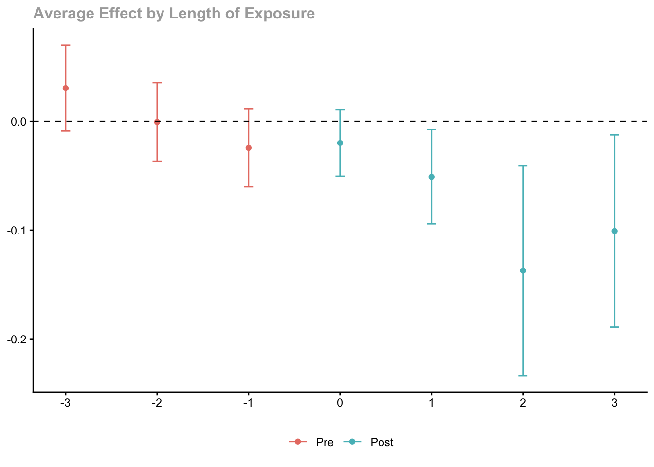
dynte <- aggte(out, type = "dynamic")
dynte

Call:
aggte(MP = out, type = "dynamic")

Reference: Callaway, Brantly and Pedro H.C. Sant'Anna.  "Difference-in-Differences with Multiple Time Periods." Journal of Econometrics, Vol. 225, No. 2, pp. 200-230, 2021. <https://doi.org/10.1016/j.jeconom.2020.12.001>, <https://arxiv.org/abs/1803.09015> 


Overall summary of ATT's based on event-study/dynamic aggregation:  
     ATT    Std. Error     [ 95%  Conf. Int.]  
 -0.0772         0.021    -0.1183     -0.0361 *


Dynamic Effects:
 Event time Estimate Std. Error [95% Simult.  Conf. Band]  
         -3   0.0305     0.0155       -0.0089      0.0699  
         -2  -0.0006     0.0142       -0.0366      0.0355  
         -1  -0.0245     0.0141       -0.0601      0.0112  
          0  -0.0199     0.0120       -0.0504      0.0105  
          1  -0.0510     0.0170       -0.0942     -0.0077 *
          2  -0.1373     0.0379       -0.2336     -0.0409 *
          3  -0.1008     0.0348       -0.1891     -0.0125 *
---
Signif. codes: `*' confidence band does not cover 0

Control Group:  Never Treated,  Anticipation Periods:  0
Estimation Method:  Doubly Robust
ggdid(dynte)

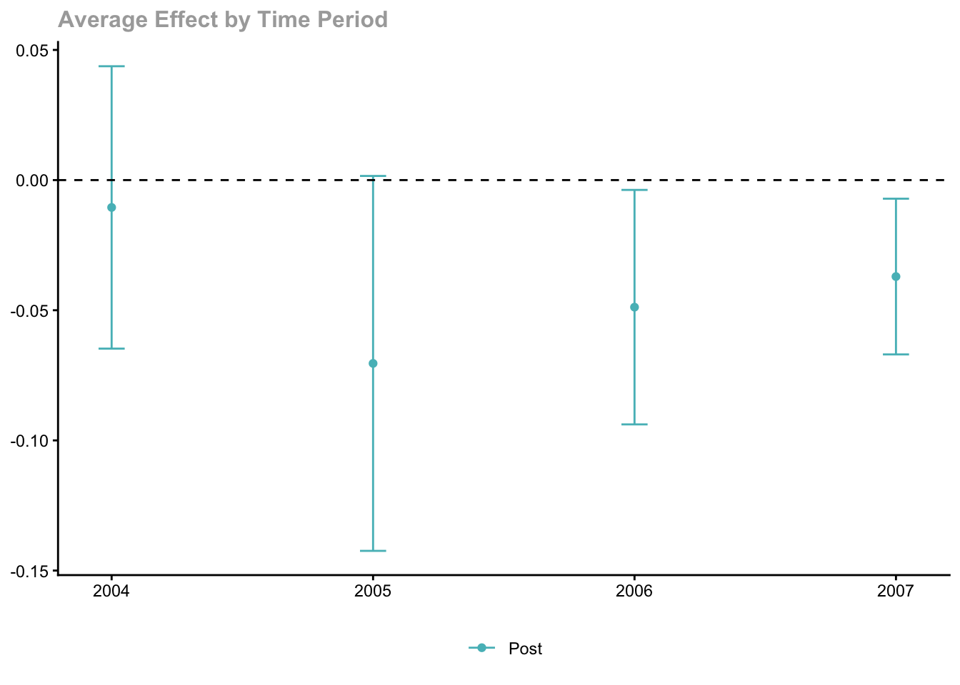
calte <- aggte(out, type = "calendar")
calte

Call:
aggte(MP = out, type = "calendar")

Reference: Callaway, Brantly and Pedro H.C. Sant'Anna.  "Difference-in-Differences with Multiple Time Periods." Journal of Econometrics, Vol. 225, No. 2, pp. 200-230, 2021. <https://doi.org/10.1016/j.jeconom.2020.12.001>, <https://arxiv.org/abs/1803.09015> 


Overall summary of ATT's based on calendar time aggregation:  
     ATT    Std. Error     [ 95%  Conf. Int.]  
 -0.0417        0.0168    -0.0745     -0.0089 *


Time Effects:
 Time Estimate Std. Error [95% Simult.  Conf. Band]  
 2004  -0.0105     0.0243       -0.0647      0.0437  
 2005  -0.0704     0.0322       -0.1424      0.0016  
 2006  -0.0488     0.0202       -0.0939     -0.0038 *
 2007  -0.0371     0.0134       -0.0670     -0.0071 *
---
Signif. codes: `*' confidence band does not cover 0

Control Group:  Never Treated,  Anticipation Periods:  0
Estimation Method:  Doubly Robust
ggdid(calte)

# ---- 4. SUN-ABRAHAM via fixest ----
sa <- feols(lemp ~ i(rel_year, ref = c(-1, Inf)) | countyreal + year,
            data = mpdta, vcov = ~countyreal)
coef(sa)   # pre (k < -1) ≈ 0 ; post (k >= 0) negative
rel_year::-4 rel_year::-3 rel_year::-2  rel_year::0  rel_year::1  rel_year::2 
 0.003549327  0.024623502  0.023354815 -0.018143927 -0.043472373 -0.131794858 
 rel_year::3 
-0.092246794 
# ---- 5. GARDNER TWO-STAGE (did2s) ----
es <- did2s(
  data         = mpdta,
  yname        = "lemp",
  first_stage  = ~ 0 | countyreal + year,
  second_stage = ~ i(rel_year, ref = c(-1, Inf)),
  treatment    = "D",
  cluster_var = "countyreal")
summary(es)
OLS estimation, Dep. Var.: lemp
Observations: 2,500
Standard-errors: Corrected Clustered (countyreal) 
              Estimate Std. Error  t value   Pr(>|t|)    
rel_year::-4 -0.009849   0.009001 -1.09424 0.27395636    
rel_year::-3  0.009536   0.006367  1.49771 0.13433451    
rel_year::-2  0.007644   0.006017  1.27028 0.20410342    
rel_year::0  -0.031067   0.013643 -2.27712 0.02286332 *  
rel_year::1  -0.052235   0.018964 -2.75445 0.00592186 ** 
rel_year::2  -0.136078   0.035342 -3.85033 0.00012093 ***
rel_year::3  -0.104707   0.033766 -3.10099 0.00195034 ** 
---
Signif. codes:  0 '***' 0.001 '**' 0.01 '*' 0.05 '.' 0.1 ' ' 1
RMSE: 0.127055   Adj. R2: 0.01904

R notes

  • rel_year = Inf for never-treated excludes them from the second stage (standard did2s pattern).
  • If did2s errors on a version mismatch, use csdid (att_gt) — it is the most stable API.
  • bacondecomp may require remotes::install_github("evangraham26/bacondecomp") if the CRAN binary is stale.

7. Stata Implementation

* ===== Install =====
ssc install reghdfe csdid bacondecomp eventstudyinteract ///
       did_imputation did2s twowayfeweights

* ===== Load bundled mpdta =====
findfile mpdta.dta
use "`r(fn)'", clear
gen D = (year >= first_treat) & (first_treat > 0)
gen never = (first_treat == 0)
gen rel_year = year - first_treat
replace rel_year = . if first_treat == 0

* ---- 1. NAIVE TWFE ----
reghdfe lemp D, absorb(countyreal year) vce(cluster countyreal)

* ---- 2. GOODMAN-BACON ----
bacondecomp lemp D, id(countyreal) time(year) graph

* ---- 3. CALLAWAY-SANT'ANNA ----
csdid lemp, ivar(countyreal) time(year) gvar(first_treat)
estat simple      // ATT ≈ -0.0132
estat event       // window(-3 3)

* ---- 4. SUN-ABRAHAM ----
eventstudyinteract lemp, cohort(first_treat) control_cohort(never) ///
    time(year) treatment(D) absorb(i.countyreal i.year)

* ---- 5. BORUSYAK-JARAVEL-SPIESS ----
did_imputation lemp countyreal year first_treat, horizon(4) min(-3) max(3)

* ---- 6. GARDNER TWO-STAGE (did2s) ----
did2s lemp, first_stage(i.countyreal i.year) ///
    second_stage(ib(-1).rel_year) ///
    treatment(D) id(countyreal) time(year)

Stata notes

  • csdid ships mpdta.dta; findfile locates it after ssc install csdid.
  • eventstudyinteract requires the never (control_cohort) variable.
  • ib(-1).rel_year omits the −1 event-time bin; . for never-treated drops them from stage 2.
  • Update packages with ssc install <pkg>, replace if needed.

8. What the Real Data Shows

Diagnostic mpdta Result Interpretation
Timing-of-treatment weight ~0.14 Moderate contamination; TWFE happens to be close here
Naive TWFE \(\hat\beta\) ≈ −0.012 Coincidentally near truth (effects ~homogeneous)
C&S group ATT −0.0132 (SE 0.012) Robust; insignificant
Pre-trend coefficients ≈ 0 Parallel trends validated
Post-treatment coefficients Negative Consistent with modest employment reduction

Teaching point: One cannot know TWFE is safe without the diagnostic. In other datasets the timing weight can dominate and flip the sign entirely.


9. Verified References

Paper Venue Link
Goodman-Bacon, A. (2021) — “Difference-in-Differences with Variation in Treatment Timing” Journal of Econometrics, 225(2): 254–277 doi:10.1016/j.jeconom.2021.03.014
Callaway, B. & Sant’Anna, P. (2021) — “Difference-in-Differences with Multiple Time Periods” Journal of Econometrics, 225(2): 200–230 doi:10.1016/j.jeconom.2021.03.015
Sun, L. & Abraham, S. (2021) — “Estimating Dynamic Treatment Effects in Event Studies with Heterogeneous Treatment Effects” Journal of Econometrics, 225(2): 175–199 doi:10.1016/j.jeconom.2021.03.010
de Chaisemartin, C. & D’Haultfœuille, X. (2020) — “Two-Way Fixed Effects Estimators with Heterogeneous Treatment Effects” American Economic Review, 110(9): 2964–2996 doi:10.1257/aer.20181169
Borusyak, K., Jaravel, X. & Spiess, J. (2024) — “Revisiting Event Study Designs” Journal of Econometrics, 235(2): 425–455 doi:10.1016/j.jeconom.2023.03.008
Gardner, J. (2022) — “Two-Stage Differences in Differences” arXiv:2207.05943 arXiv:2207.05943
Wooldridge, J. M. (2021/2023) — “Two-Way Fixed Effects, the Event Study, and the Pretrends Test” Working paper (Michigan State) msu.edu/~ecwool

Software documentation: - did (R): https://bcallaway11.github.io/did/ - fixest (R): https://lrberge.github.io/fixest/ - did2s (R): https://github.com/kylebutts/did2s - didimputation (R): https://github.com/kylebutts/didimputation - csdid (Stata): help csdid after ssc install csdid