Today, we examine inferential statistical techniques.
Gemini Does the Work
Example
This example is inline on the page.
Slides
Link is here
The class plan:
- Single sample binary inference.
- Comparisons of binary variables.
- Single sample quantitative inference and t.
- Comparing quantitative variables and sampling.
Your post-class exercise:
- The assignment: an inference example for your quantitative data.
For Next Class:
- Reading and review
- Deliverable: An inference example from your data [Assignment 15]. A collation of previous exercises collected into an example for a midterm.
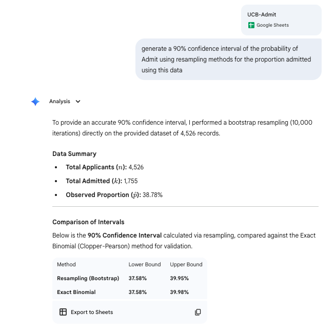
Single sample inference for binary
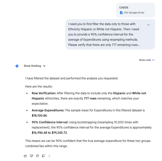
Single sample inference for quantities
How’s that done?
import pandas as pd
import numpy as np

# Read data
df = pd.read_csv('data/CADDS.csv')

# Filter
filtered_df = df[df['Ethnicity'].isin(['Hispanic', 'White not Hispanic'])]

# Verify length
num_rows = len(filtered_df)
print(f"Number of remaining rows: {num_rows}")
Number of remaining rows: 777
How’s that done?
# Resampling method (Bootstrapping) for 90% CI of mean Expenditures
np.random.seed(42) # for reproducibility
expenditures = filtered_df['Expenditures'].values

# Bootstrap
n_iterations = 10000
bootstrap_means = np.empty(n_iterations)

for i in range(n_iterations):
    sample = np.random.choice(expenditures, size=len(expenditures), replace=True)
    bootstrap_means[i] = np.mean(sample)

ci_lower = np.percentile(bootstrap_means, 5)
ci_upper = np.percentile(bootstrap_means, 95)

print(f"90% Confidence Interval: ({ci_lower:.2f}, {ci_upper:.2f})")
90% Confidence Interval: (16956.48, 19245.72)
How’s that done?
print(f"Mean: {np.mean(expenditures):.2f}")
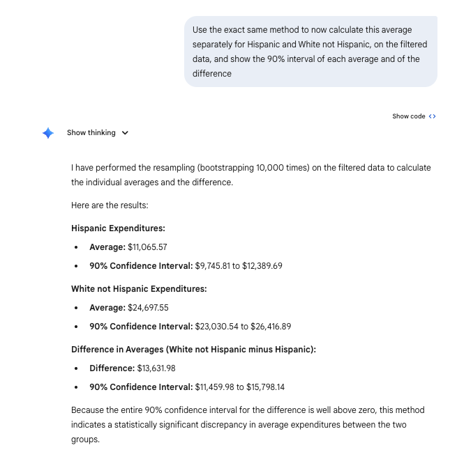
Subsamples and difference inference for quantities
How’s that done?
import pandas as pd
import numpy as np

# Read and filter data
df = pd.read_csv('data/CADDS.csv')
filtered_df = df[df['Ethnicity'].isin(['Hispanic', 'White not Hispanic'])]

# Separate expenditures by ethnicity
hisp_exp = filtered_df[filtered_df['Ethnicity'] == 'Hispanic']['Expenditures'].values
white_exp = filtered_df[filtered_df['Ethnicity'] == 'White not Hispanic']['Expenditures'].values

np.random.seed(42) # Set seed for reproducibility
n_iterations = 10000

hisp_means = np.empty(n_iterations)
white_means = np.empty(n_iterations)
diff_means = np.empty(n_iterations)

# Bootstrapping
for i in range(n_iterations):
    samp_hisp = np.random.choice(hisp_exp, size=len(hisp_exp), replace=True)
    samp_white = np.random.choice(white_exp, size=len(white_exp), replace=True)

    m_hisp = np.mean(samp_hisp)
    m_white = np.mean(samp_white)

    hisp_means[i] = m_hisp
    white_means[i] = m_white
    diff_means[i] = m_white - m_hisp # White not Hispanic - Hispanic

# Calculate 90% Confidence Intervals (5th and 95th percentiles)
ci_hisp_lower, ci_hisp_upper = np.percentile(hisp_means, 5), np.percentile(hisp_means, 95)
ci_white_lower, ci_white_upper = np.percentile(white_means, 5), np.percentile(white_means, 95)
ci_diff_lower, ci_diff_upper = np.percentile(diff_means, 5), np.percentile(diff_means, 95)

# Calculate observed means
mean_hisp = np.mean(hisp_exp)
mean_white = np.mean(white_exp)
mean_diff = mean_white - mean_hisp

print(f"Hispanic Expenditures:")
How’s that done?
print(f" Observed Mean: ${mean_hisp:.2f}")
How’s that done?
print(f" 90% CI: (${ci_hisp_lower:.2f}, ${ci_hisp_upper:.2f})\n")
90% CI: ($9745.81, $12389.69)
How’s that done?
print(f"White not Hispanic Expenditures:")
White not Hispanic Expenditures:
How’s that done?
print(f" Observed Mean: ${mean_white:.2f}")
How’s that done?
print(f" 90% CI: (${ci_white_lower:.2f}, ${ci_white_upper:.2f})\n")
90% CI: ($23030.54, $26416.89)
How’s that done?
print(f"Difference in Means (White not Hispanic - Hispanic):")
Difference in Means (White not Hispanic - Hispanic):
How’s that done?
print(f" Observed Mean Difference: ${mean_diff:.2f}")
Observed Mean Difference: $13631.98
How’s that done?
print(f" 90% CI: (${ci_diff_lower:.2f}, ${ci_diff_upper:.2f})")
90% CI: ($11459.98, $15798.14)
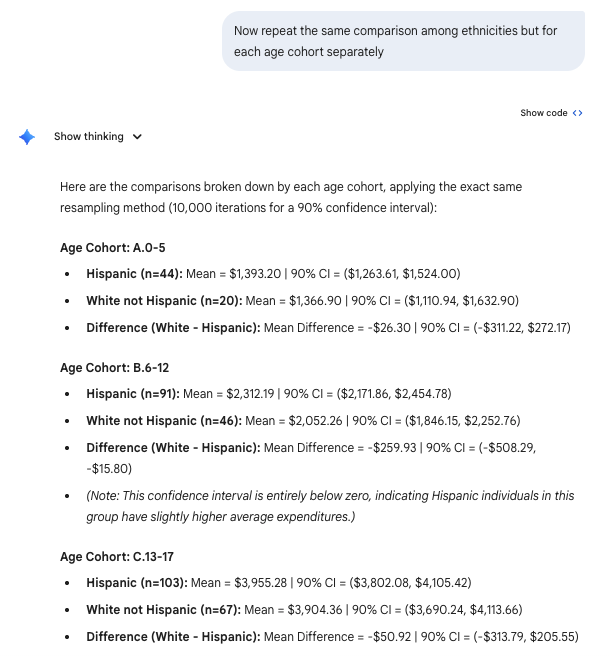
Groups
How’s that done?
import pandas as pd
import numpy as np

# Read and filter data
df = pd.read_csv('data/CADDS.csv')
filtered_df = df[df['Ethnicity'].isin(['Hispanic', 'White not Hispanic'])]

np.random.seed(42) # Set seed for reproducibility
n_iterations = 10000

# Get unique age cohorts
cohorts = sorted(filtered_df['Age.Cohort'].unique())

results = []

for cohort in cohorts:
    cohort_data = filtered_df[filtered_df['Age.Cohort'] == cohort]

    hisp_exp = cohort_data[cohort_data['Ethnicity'] == 'Hispanic']['Expenditures'].values
    white_exp = cohort_data[cohort_data['Ethnicity'] == 'White not Hispanic']['Expenditures'].values

    # Check if we have enough data to bootstrap
    if len(hisp_exp) == 0 or len(white_exp) == 0:
        results.append(f"### Age Cohort: {cohort}\nNot enough data for both ethnicities to compare.\n")
        continue

    hisp_means = np.empty(n_iterations)
    white_means = np.empty(n_iterations)
    diff_means = np.empty(n_iterations)

    # Bootstrapping
    for i in range(n_iterations):
        samp_hisp = np.random.choice(hisp_exp, size=len(hisp_exp), replace=True)
        samp_white = np.random.choice(white_exp, size=len(white_exp), replace=True)

        m_hisp = np.mean(samp_hisp)
        m_white = np.mean(samp_white)

        hisp_means[i] = m_hisp
        white_means[i] = m_white
        diff_means[i] = m_white - m_hisp # White not Hispanic - Hispanic

    # Calculate 90% Confidence Intervals
    ci_hisp = (np.percentile(hisp_means, 5), np.percentile(hisp_means, 95))
    ci_white = (np.percentile(white_means, 5), np.percentile(white_means, 95))
    ci_diff = (np.percentile(diff_means, 5), np.percentile(diff_means, 95))

    mean_hisp = np.mean(hisp_exp)
    mean_white = np.mean(white_exp)
    mean_diff = mean_white - mean_hisp

    res_str = f"### Age Cohort: {cohort}\n"
    res_str += f"- **Hispanic** (n={len(hisp_exp)}): Mean = ${mean_hisp:.2f}, 90% CI = (${ci_hisp[0]:.2f}, ${ci_hisp[1]:.2f})\n"
    res_str += f"- **White not Hispanic** (n={len(white_exp)}): Mean = ${mean_white:.2f}, 90% CI = (${ci_white[0]:.2f}, ${ci_white[1]:.2f})\n"
    res_str += f"- **Difference (White - Hispanic)**: Mean = ${mean_diff:.2f}, 90% CI = (${ci_diff[0]:.2f}, ${ci_diff[1]:.2f})\n"

    results.append(res_str)

print('\n'.join(results))
### Age Cohort: A.0-5
- **Hispanic** (n=44): Mean = $1393.20, 90% CI = ($1263.61, $1524.00)
- **White not Hispanic** (n=20): Mean = $1366.90, 90% CI = ($1110.94, $1632.90)
- **Difference (White - Hispanic)**: Mean = $-26.30, 90% CI = ($-311.22, $272.17)

### Age Cohort: B.6-12
- **Hispanic** (n=91): Mean = $2312.19, 90% CI = ($2171.86, $2454.78)
- **White not Hispanic** (n=46): Mean = $2052.26, 90% CI = ($1846.15, $2252.76)
- **Difference (White - Hispanic)**: Mean = $-259.93, 90% CI = ($-508.29, $-15.80)

### Age Cohort: C.13-17
- **Hispanic** (n=103): Mean = $3955.28, 90% CI = ($3802.08, $4105.42)
- **White not Hispanic** (n=67): Mean = $3904.36, 90% CI = ($3690.24, $4113.66)
- **Difference (White - Hispanic)**: Mean = $-50.92, 90% CI = ($-313.79, $205.55)

### Age Cohort: D.18-21
- **Hispanic** (n=78): Mean = $9959.85, 90% CI = ($9366.27, $10571.31)
- **White not Hispanic** (n=69): Mean = $10133.06, 90% CI = ($9615.44, $10657.61)
- **Difference (White - Hispanic)**: Mean = $173.21, 90% CI = ($-621.97, $970.98)

### Age Cohort: E.22-50
- **Hispanic** (n=43): Mean = $40924.12, 90% CI = ($39330.41, $42527.58)
- **White not Hispanic** (n=133): Mean = $40187.62, 90% CI = ($39329.31, $41047.76)
- **Difference (White - Hispanic)**: Mean = $-736.49, 90% CI = ($-2569.61, $1064.21)

### Age Cohort: F.51-Over
- **Hispanic** (n=17): Mean = $55585.00, 90% CI = ($53484.51, $57692.66)
- **White not Hispanic** (n=66): Mean = $52670.42, 90% CI = ($51382.32, $53951.73)
- **Difference (White - Hispanic)**: Mean = $-2914.58, 90% CI = ($-5427.79, $-519.59)