The midterm: Review the assignments and bring yourself to speed with them. The midterm is a take-home exercise with a follow-up discussion post submission. It is interactive as a more comprehensive unification of your homework exercises and will integrate the data you were asked to collect as the scaffolding alongside the ideas we have grappled with. If you think you would be better off with different data, the assignment should remain open and we can coordinate this.
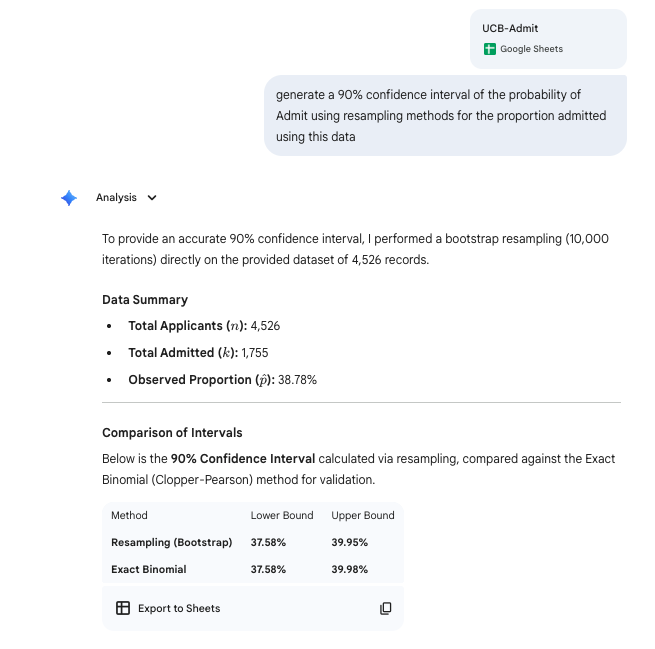
Single sample inference for binary
Inference 1
Single sample inference for quantities
Inference 2
How’s that done?
import pandas as pdimport numpy as np# Read datadf = pd.read_csv('data/CADDS.csv')# Filterfiltered_df = df[df['Ethnicity'].isin(['Hispanic', 'White not Hispanic'])]# Verify lengthnum_rows =len(filtered_df)print(f"Number of remaining rows: {num_rows}")
Number of remaining rows: 777
How’s that done?
# Resampling method (Bootstrapping) for 90% CI of mean Expendituresnp.random.seed(42) # for reproducibilityexpenditures = filtered_df['Expenditures'].values# Bootstrapn_iterations =10000bootstrap_means = np.empty(n_iterations)for i inrange(n_iterations): sample = np.random.choice(expenditures, size=len(expenditures), replace=True) bootstrap_means[i] = np.mean(sample)ci_lower = np.percentile(bootstrap_means, 5)ci_upper = np.percentile(bootstrap_means, 95)print(f"90% Confidence Interval: ({ci_lower:.2f}, {ci_upper:.2f})")
90% Confidence Interval: (16956.48, 19245.72)
How’s that done?
print(f"Mean: {np.mean(expenditures):.2f}")
Mean: 18100.86
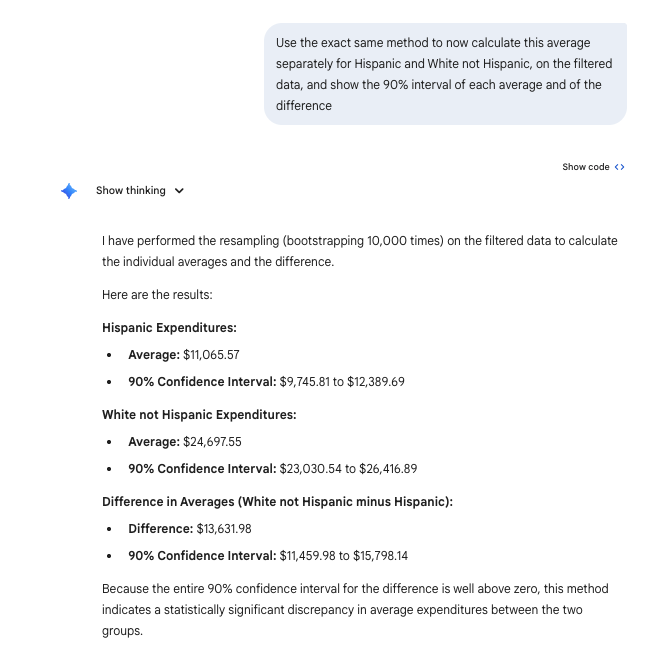
Subsamples and difference inference for quantities
Inference 3
How’s that done?
import pandas as pdimport numpy as np# Read and filter datadf = pd.read_csv('data/CADDS.csv')filtered_df = df[df['Ethnicity'].isin(['Hispanic', 'White not Hispanic'])]# Separate expenditures by ethnicityhisp_exp = filtered_df[filtered_df['Ethnicity'] =='Hispanic']['Expenditures'].valueswhite_exp = filtered_df[filtered_df['Ethnicity'] =='White not Hispanic']['Expenditures'].valuesnp.random.seed(42) # Set seed for reproducibilityn_iterations =10000hisp_means = np.empty(n_iterations)white_means = np.empty(n_iterations)diff_means = np.empty(n_iterations)# Bootstrappingfor i inrange(n_iterations): samp_hisp = np.random.choice(hisp_exp, size=len(hisp_exp), replace=True) samp_white = np.random.choice(white_exp, size=len(white_exp), replace=True) m_hisp = np.mean(samp_hisp) m_white = np.mean(samp_white) hisp_means[i] = m_hisp white_means[i] = m_white diff_means[i] = m_white - m_hisp # White not Hispanic - Hispanic# Calculate 90% Confidence Intervals (5th and 95th percentiles)ci_hisp_lower, ci_hisp_upper = np.percentile(hisp_means, 5), np.percentile(hisp_means, 95)ci_white_lower, ci_white_upper = np.percentile(white_means, 5), np.percentile(white_means, 95)ci_diff_lower, ci_diff_upper = np.percentile(diff_means, 5), np.percentile(diff_means, 95)# Calculate observed meansmean_hisp = np.mean(hisp_exp)mean_white = np.mean(white_exp)mean_diff = mean_white - mean_hispprint(f"Hispanic Expenditures:")
import pandas as pdimport numpy as np# Read and filter datadf = pd.read_csv('data/CADDS.csv')filtered_df = df[df['Ethnicity'].isin(['Hispanic', 'White not Hispanic'])]np.random.seed(42) # Set seed for reproducibilityn_iterations =10000# Get unique age cohortscohorts =sorted(filtered_df['Age.Cohort'].unique())results = []for cohort in cohorts: cohort_data = filtered_df[filtered_df['Age.Cohort'] == cohort] hisp_exp = cohort_data[cohort_data['Ethnicity'] =='Hispanic']['Expenditures'].values white_exp = cohort_data[cohort_data['Ethnicity'] =='White not Hispanic']['Expenditures'].values# Check if we have enough data to bootstrapiflen(hisp_exp) ==0orlen(white_exp) ==0: results.append(f"### Age Cohort: {cohort}\nNot enough data for both ethnicities to compare.\n")continue hisp_means = np.empty(n_iterations) white_means = np.empty(n_iterations) diff_means = np.empty(n_iterations)# Bootstrappingfor i inrange(n_iterations): samp_hisp = np.random.choice(hisp_exp, size=len(hisp_exp), replace=True) samp_white = np.random.choice(white_exp, size=len(white_exp), replace=True) m_hisp = np.mean(samp_hisp) m_white = np.mean(samp_white) hisp_means[i] = m_hisp white_means[i] = m_white diff_means[i] = m_white - m_hisp # White not Hispanic - Hispanic# Calculate 90% Confidence Intervals ci_hisp = (np.percentile(hisp_means, 5), np.percentile(hisp_means, 95)) ci_white = (np.percentile(white_means, 5), np.percentile(white_means, 95)) ci_diff = (np.percentile(diff_means, 5), np.percentile(diff_means, 95)) mean_hisp = np.mean(hisp_exp) mean_white = np.mean(white_exp) mean_diff = mean_white - mean_hisp res_str =f"### Age Cohort: {cohort}\n" res_str +=f"- **Hispanic** (n={len(hisp_exp)}): Mean = ${mean_hisp:.2f}, 90% CI = (${ci_hisp[0]:.2f}, ${ci_hisp[1]:.2f})\n" res_str +=f"- **White not Hispanic** (n={len(white_exp)}): Mean = ${mean_white:.2f}, 90% CI = (${ci_white[0]:.2f}, ${ci_white[1]:.2f})\n" res_str +=f"- **Difference (White - Hispanic)**: Mean = ${mean_diff:.2f}, 90% CI = (${ci_diff[0]:.2f}, ${ci_diff[1]:.2f})\n" results.append(res_str)print('\n'.join(results))
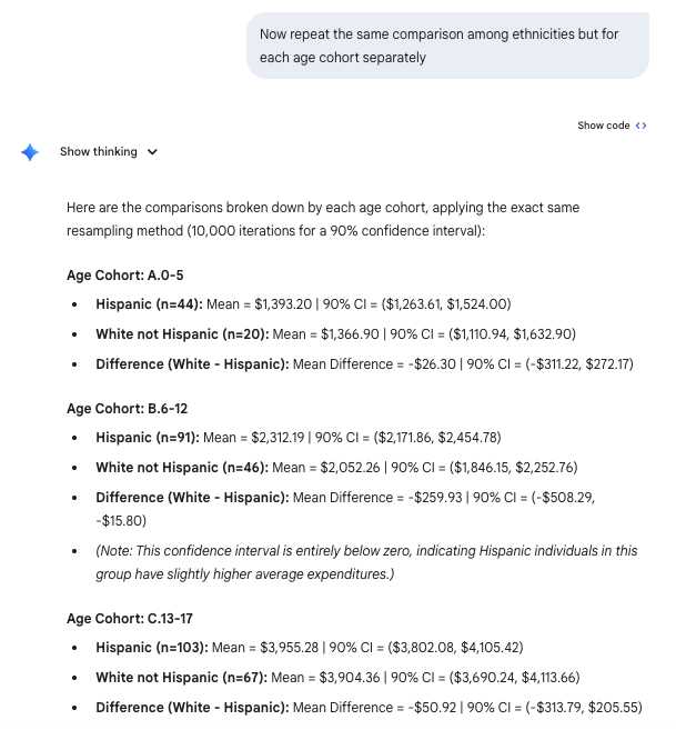
### Age Cohort: A.0-5
- **Hispanic** (n=44): Mean = $1393.20, 90% CI = ($1263.61, $1524.00)
- **White not Hispanic** (n=20): Mean = $1366.90, 90% CI = ($1110.94, $1632.90)
- **Difference (White - Hispanic)**: Mean = $-26.30, 90% CI = ($-311.22, $272.17)

### Age Cohort: B.6-12
- **Hispanic** (n=91): Mean = $2312.19, 90% CI = ($2171.86, $2454.78)
- **White not Hispanic** (n=46): Mean = $2052.26, 90% CI = ($1846.15, $2252.76)
- **Difference (White - Hispanic)**: Mean = $-259.93, 90% CI = ($-508.29, $-15.80)

### Age Cohort: C.13-17
- **Hispanic** (n=103): Mean = $3955.28, 90% CI = ($3802.08, $4105.42)
- **White not Hispanic** (n=67): Mean = $3904.36, 90% CI = ($3690.24, $4113.66)
- **Difference (White - Hispanic)**: Mean = $-50.92, 90% CI = ($-313.79, $205.55)

### Age Cohort: D.18-21
- **Hispanic** (n=78): Mean = $9959.85, 90% CI = ($9366.27, $10571.31)
- **White not Hispanic** (n=69): Mean = $10133.06, 90% CI = ($9615.44, $10657.61)
- **Difference (White - Hispanic)**: Mean = $173.21, 90% CI = ($-621.97, $970.98)

### Age Cohort: E.22-50
- **Hispanic** (n=43): Mean = $40924.12, 90% CI = ($39330.41, $42527.58)
- **White not Hispanic** (n=133): Mean = $40187.62, 90% CI = ($39329.31, $41047.76)
- **Difference (White - Hispanic)**: Mean = $-736.49, 90% CI = ($-2569.61, $1064.21)

### Age Cohort: F.51-Over
- **Hispanic** (n=17): Mean = $55585.00, 90% CI = ($53484.51, $57692.66)
- **White not Hispanic** (n=66): Mean = $52670.42, 90% CI = ($51382.32, $53951.73)
- **Difference (White - Hispanic)**: Mean = $-2914.58, 90% CI = ($-5427.79, $-519.59)
Compare
Paired Comparison
Prompt: I need to compare with and without in the following data. I need a paired comparison of the batches along with appropriate summaries to confirm the data were appropriately entered.
CONCRETE BATCH COMPARISON REPORT
DATA VERIFICATION & INTEGRITY A row-by-row verification was performed: Difference = (No Additive) - (Additive).
Entry Check: Complete. All calculated values match the provided data.
CONCLUSION: The p-value (0.015) is less than 0.05, indicating a statistically significant increase in values when the additive is used. On average, the additive improves the measurement by approximately 158.33 units.