On Probability
OIS Chapter 3 and Jaynes
Overview
- The ECDF.
- Tables
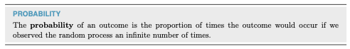
- Probability
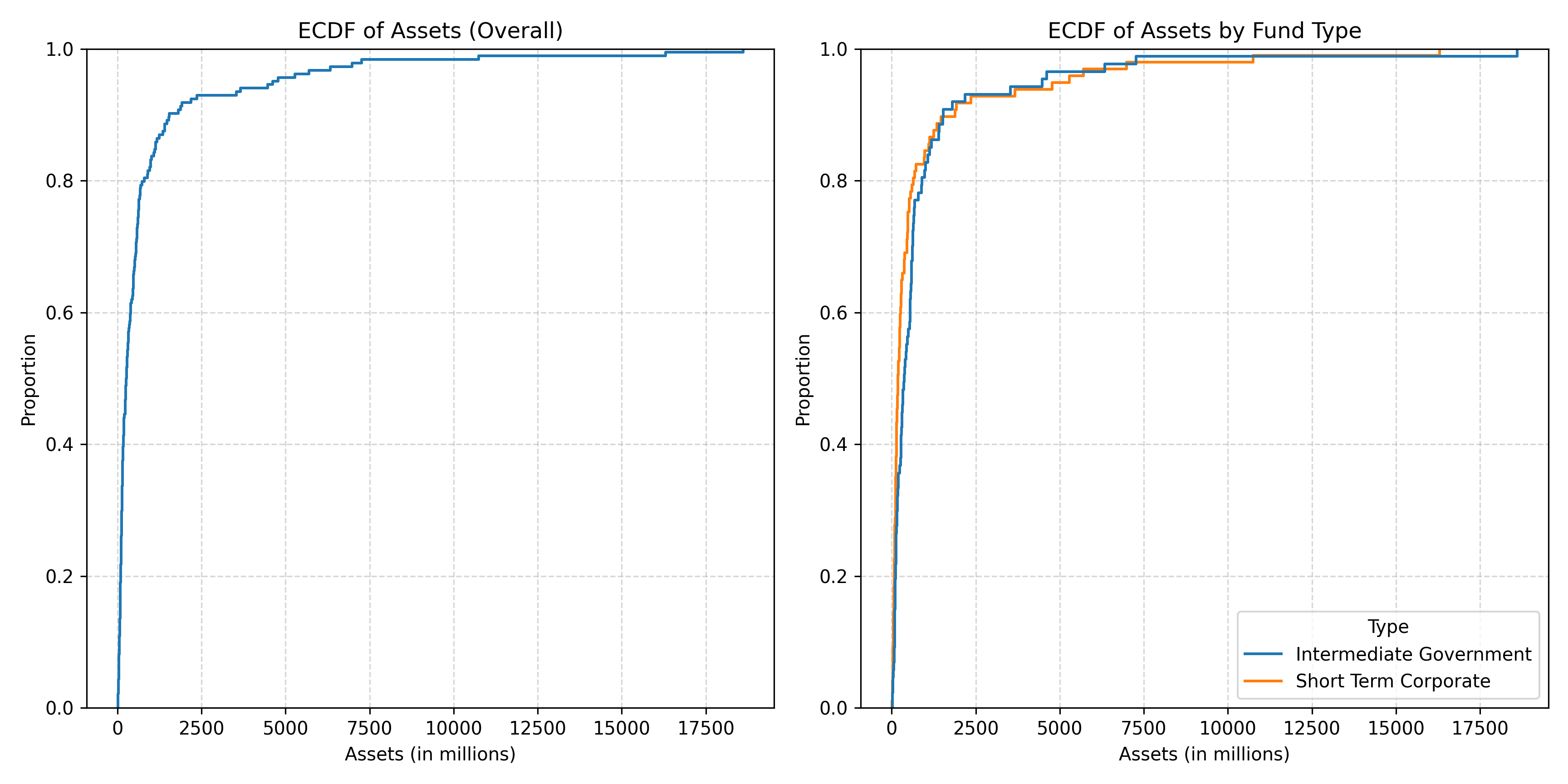
ECDFs and Probability: A Link
Empirical Cumulative Distribution Functions * the y-axis is always a proportion [0-1]/percentage [0/100].
Probability and Tables
Probability
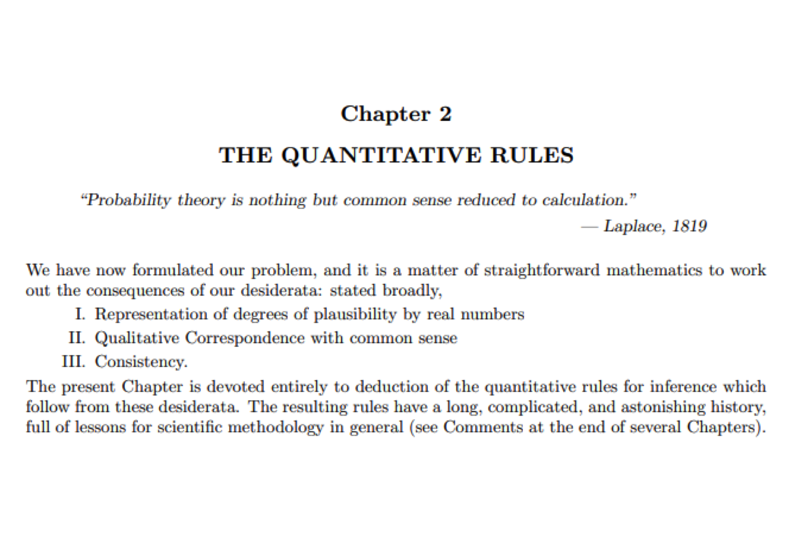
Why Jaynes?
His approach is intuitive. If you are familiar with probability already, some of you have formal training, Appendix A sets out the key differences. The nominal assignment is to read this with the assistance of NotebookLM and Gemini. It is not the easiest, but his ideas on subjective probability are important.
Why did I ask you to read this? He builds a basic foundation. He derives rules. Those rules are the same rules that we will deploy. But he does it from more basic foundations. Yes, he can do math. That’s not the point; there is a simple representation of all of these ideas. And only a small number of rules that we will define precisely.
His books taught me a great deal, personally.
Probability
Two rules:
- Probabilities sum to one.
- The probability of any event is greater than or equal to zero.
Where does Probability Come From?
There are three common sources of probabilities:
- Known formula [Dice, Coins, etc.]
- Empirical frequency
- Subjective belief
Jaynes is a proponent of the latter.
The Book
The infinity bit is opinionated. Hence the reliance on the law of large numbers.
A priori probability
The probability of a given integer on a k-sided die: \(\frac{1}{k}\).
The probability of heads with a fair coin: \(\frac{1}{2}\).
The probability of a Queen? \(\frac{4}{52}\)
The probability of a Diamond? \(\frac{13}{52}\)
The Queen of Diamonds? \(\frac{1}{52}\) or \((\frac{4}{52}\times\frac{13}{52})\)
Quasirandom numbers
Empirical probability: frequency
How often does something happen?
This is Historical Statistics
How likely am I to be admitted? Consult the admissions rate
How fast do I drive? Likelihood of law enforcement and need for speed
In data: this is tables.
Berkeley
           No  Yes
  Female 1278  557
  Male   1493 1198
M.F No Yes
Female 1278 557
Male 1493 1198How’s that done?
library(tidyverse)
library(janitor)
table(UCBAdmit$M.F,UCBAdmit$Admit)
UCBAdmit %>% tabyl(M.F, Admit)
Three Versions
How’s that done?
prop.table(table(UCBAdmit$M.F,UCBAdmit$Admit), 1)
                No       Yes
  Female 0.6964578 0.3035422
  Male   0.5548123 0.4451877
How’s that done?
prop.table(table(UCBAdmit$M.F,UCBAdmit$Admit), 2)
                No       Yes
  Female 0.4612053 0.3173789
  Male   0.5387947 0.6826211
How’s that done?
prop.table(table(UCBAdmit$M.F,UCBAdmit$Admit))
                No       Yes
  Female 0.2823685 0.1230667
  Male   0.3298719 0.2646929
How’s that done?
UCBAdmit %>% tabyl(M.F, Admit) %>% adorn_percentages("row") M.F No Yes
Female 0.6964578 0.3035422
Male 0.5548123 0.4451877How’s that done?
UCBAdmit %>% tabyl(M.F, Admit) %>% adorn_percentages("col") M.F No Yes
Female 0.4612053 0.3173789
Male 0.5387947 0.6826211How’s that done?
UCBAdmit %>% tabyl(M.F, Admit) %>% adorn_percentages("all") M.F No Yes
Female 0.2823685 0.1230667
Male 0.3298719 0.2646929Plot It
How’s that done?
( UCBM <- ggplot(UCBAdmit) + aes(x=M.F, fill=Admit) + geom_bar(position="dodge") + scale_fill_viridis_d() )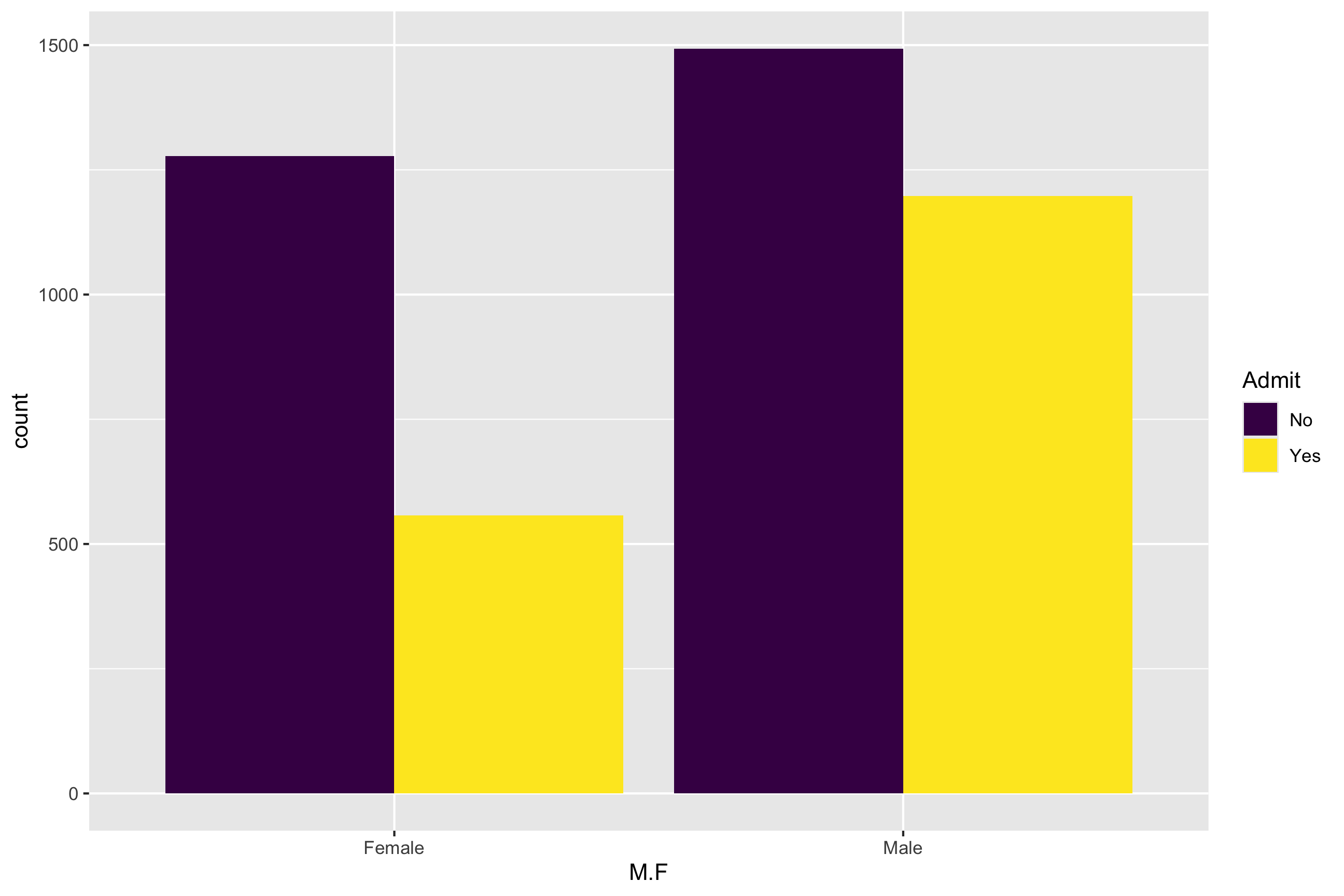
Subjective Probability
How likely do we believe something is?
The Great Divide
Empirical frequency vs. subjective belief
Empirical Frequency: She’s Right
Physics Disagrees: We Goin Nova…..
Annie’s a liar.
What matters in group decision making is probably as much the beliefs [subjective] as the evidence [frequency].
How should we reflect this in strategies of argumentation/persuasion?
Think
What matters?
Disjoint events/mutual exclusivity
Outcomes are called disjoint or mutually exclusive if they cannot both occur.
Three Concepts from Set Theory
- Intersection [and]
- Union [or] avoid double counting the intersection
- Complement [not]
Three Distinct Probabilities
- Joint: Pr(x=x and y=y)
- Marginal: Pr(x=x) or Pr(y=y)
- Conditional: Pr(x=x | y=y) or Pr(y =y | x = x)
Joint Probability
The table sums to one.
For Berkeley:
How’s that done?
UCBAdmit %>% tabyl(M.F, Admit) %>% adorn_percentages("all") M.F No Yes
Female 0.2823685 0.1230667
Male 0.3298719 0.2646929How’s that done?
prop.table(table(UCBAdmit$M.F,UCBAdmit$Admit))
                No       Yes
  Female 0.2823685 0.1230667
  Male   0.3298719 0.2646929
Marginal Probability
The row/column sums to one. We collapse the table to a single margin. Here, two can be identified. The probability of Admit and the probability of M.F.
How’s that done?
UCBAdmit %>% tabyl(M.F) M.F n percent
Female 1835 0.4054353
Male 2691 0.5945647How’s that done?
UCBAdmit %>% tabyl(Admit) Admit n percent
No 2771 0.6122404
Yes 1755 0.3877596How’s that done?
prop.table(table(UCBAdmit$M.F))
   Female      Male
0.4054353 0.5945647
How’s that done?
prop.table(table(UCBAdmit$Admit))
       No       Yes
0.6122404 0.3877596
Conditional Probability
How does one margin of the table break down given values of another? Each row or column sums to one
Four can be identified, the probability of admission/rejection for Male, for Female; the probability of male or female for admits/rejects.
For Berkeley:
How’s that done?
UCBAdmit %>% tabyl(M.F, Admit) %>% adorn_percentages("row") M.F No Yes
Female 0.6964578 0.3035422
Male 0.5548123 0.4451877How’s that done?
prop.table(table(UCBAdmit$M.F,UCBAdmit$Admit), 1)
                No       Yes
  Female 0.6964578 0.3035422
  Male   0.5548123 0.4451877
How’s that done?
UCBAdmit %>% tabyl(M.F, Admit) %>% adorn_percentages("col") M.F No Yes
Female 0.4612053 0.3173789
Male 0.5387947 0.6826211How’s that done?
prop.table(table(UCBAdmit$M.F,UCBAdmit$Admit), 2)
                No       Yes
  Female 0.4612053 0.3173789
  Male   0.5387947 0.6826211
Law of Total Probability
Is a combination of the distributive property of multiplication and the fact that probabilities sum to one.
For example, the probability of Admitted and Male is the probability of admission for males times the probability of male.
\[ Pr(x=x, y=y) = Pr(y | x)Pr(x) \]
Or it is the probability of being admitted times the probabilty of being male among admits.
\[ Pr(x=x, y=y) = Pr(x | y)Pr(y) \]
Now the Substance
The ggplot fill aesthetic is great for displaying these things. For example, are males and females equally likely to be admitted to Berkeley?
Plaintiffs say no.
How’s that done?
ggplot(UCBAdmit) + aes(x=M.F, fill=Admit) + geom_bar() + scale_fill_viridis_d()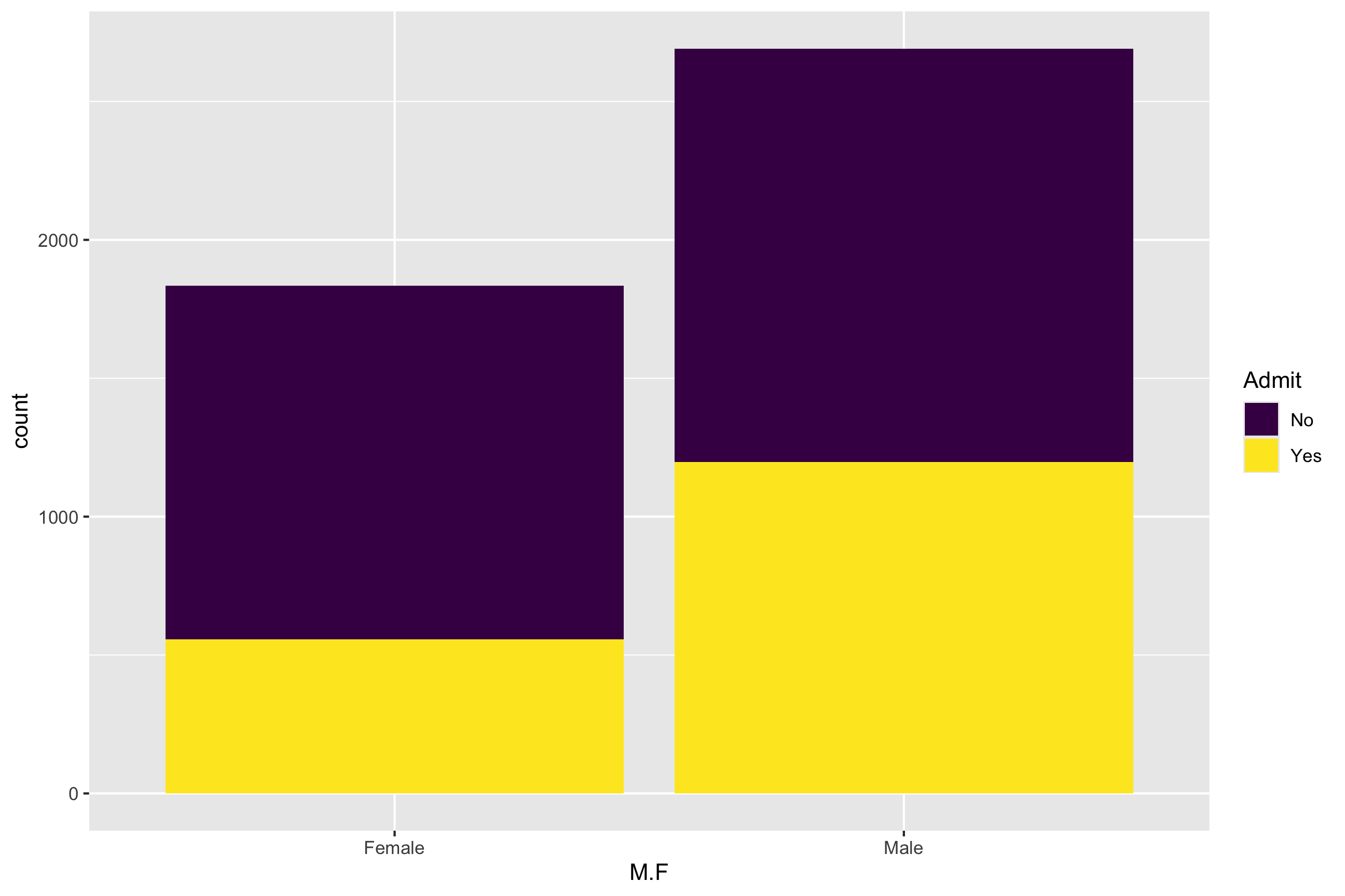
Is that an Adequate Comparison?
The University says no. Why? The most important factor in the probability of admission is likely to be the department. This has a huge impact on what we see.
How’s that done?
ggplot(UCBAdmit) +
  aes(x=M.F, fill=Admit) +
  geom_bar(position="fill") +
  scale_fill_viridis_d() +
  facet_wrap(vars(Dept))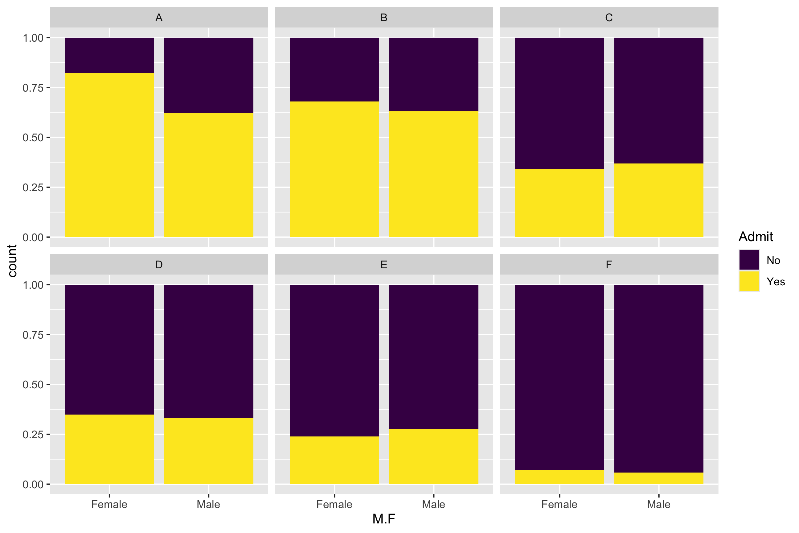
The Magic of Bayes Rule
To find the joint probability [the intersection] of x and y, we can use either of the aforementioned methods. To turn this into a conditional probability, we simply take it is a proportion of the relevant margin.
\[ Pr(x | y) = \frac{Pr(y | x) Pr(x)}{Pr(y)} \]
Applications of these Topics
A Bit on Juries
- Start from Section 3.2.7
- The juror’s decision tree
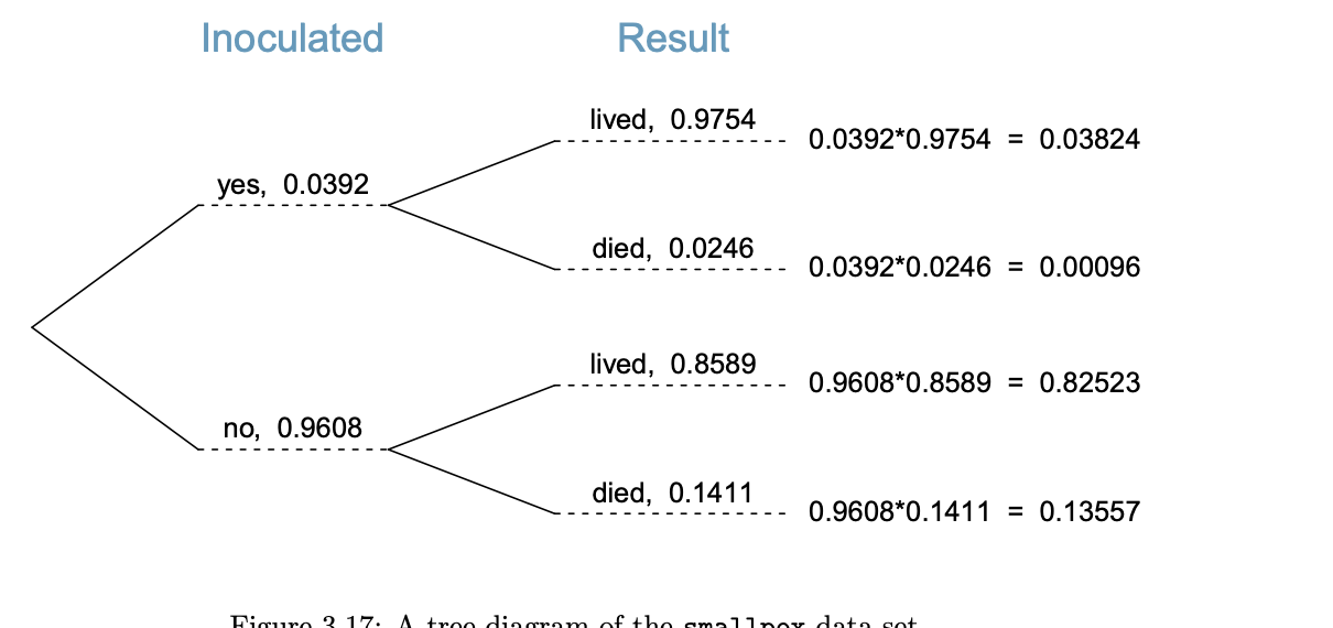
Three nodes: guilty and not at each, convict at the third.
Bayesian Reasoning is Core to Decisions with Data
\[ Pr(Decision | data) = \frac{Pr(data | Decision) Pr(Decision)}{Pr(Data)} \]