How’s that done?
# install.packages("rnaturalearth")
library(rnaturalearth)
library(tidyverse)
library(ggthemes)
library(plotly)
worldmap <- ne_download(scale = 110,
type = "countries",
category = "cultural",
destdir = tempdir(),
load = TRUE,
returnclass = "sf")
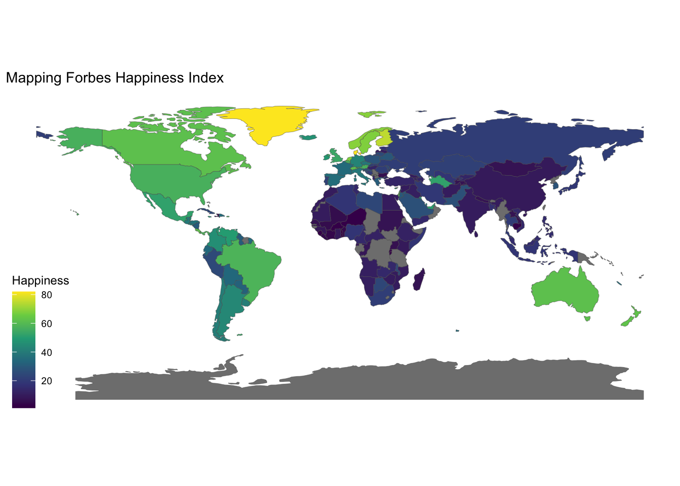
left_join(worldmap, Happiness, by=c("SOVEREIGNT" = "COUNTRY")) -> WM.Happy
There’s the data. Now for esquisse…
How’s that done?
ggplot(WM.Happy) +
 aes(fill = HAPPY, text = SOVEREIGNT) +
 geom_sf(size = 0.1) +
 scale_fill_viridis_c() +
 theme_map() + labs(title="Mapping Forbes Happiness Index", fill="Happiness") -> My.GGP
My.GGP
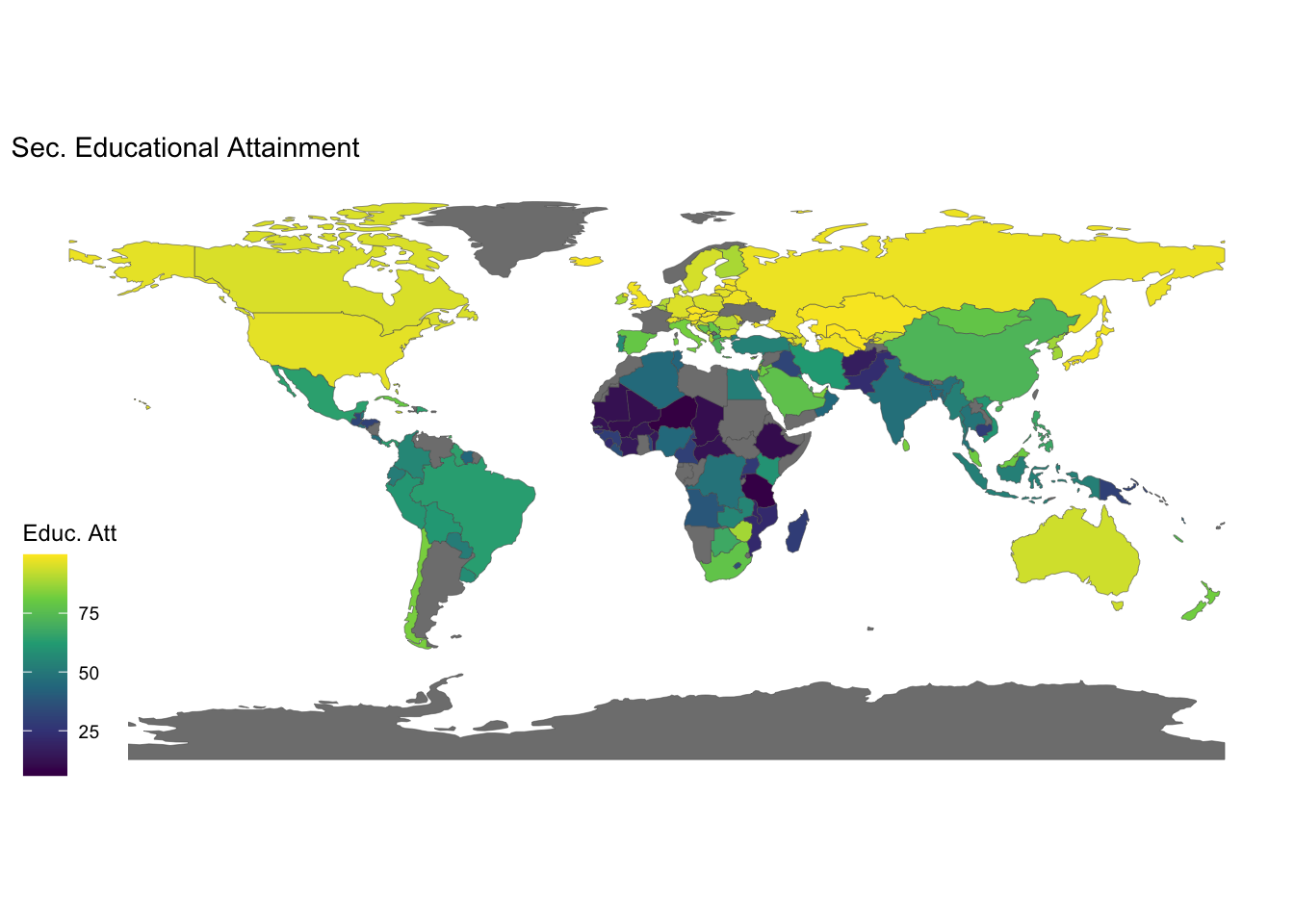
WDI
How’s that done?
library(WDI)
EdAtt1 <- WDI(country="all", indicator=c("SE.SEC.CUAT.LO.ZS"), start=2018, end=2020) |> group_by(iso3c) |> summarise(Sec.Edu.Att = mean(SE.SEC.CUAT.LO.ZS, na.rm=TRUE))
WM.EA <- left_join(worldmap, EdAtt1, by=c("ISO_A3" = "iso3c"))
ggplot(WM.EA) +
 aes(fill = Sec.Edu.Att) +
 geom_sf(size = 0.1) +
 scale_fill_viridis_c() +
 theme_map() + labs(title="Sec. Educational Attainment", fill="Educ. Att")
How’s that done?
EdAtt1 <- WDI(country="all", indicator=c("DT.DOD.PVLX.EX.ZS"), start=2018, end=2020) |> group_by(iso3c) |> summarise(Series.Mean = mean(DT.DOD.PVLX.EX.ZS, na.rm=TRUE))
tempf <- left_join(worldmap, EdAtt1, by=c("ISO_A3" = "iso3c"))
ggplot(tempf) +
 aes(fill = Series.Mean) +
 geom_sf(size = 0.1) +
 scale_fill_viridis_c() +
 theme_map() + labs(title="External Debt pc", fill="Debt")
Using Eurostat
How’s that done?
library(kableExtra)
library(eurostat)
toc <- get_eurostat_toc()
kable(search_eurostat("migrant", column = "code")) |> kableExtra::scroll_box(width="80%")
| NA |
NA |
NA |
NA |
NA |
NA |
NA |
NA |
NA |
| :----- |
:---- |
:---- |
:------------------- |
:--------------------------- |
:---------- |
:-------- |
------: |
---------: |
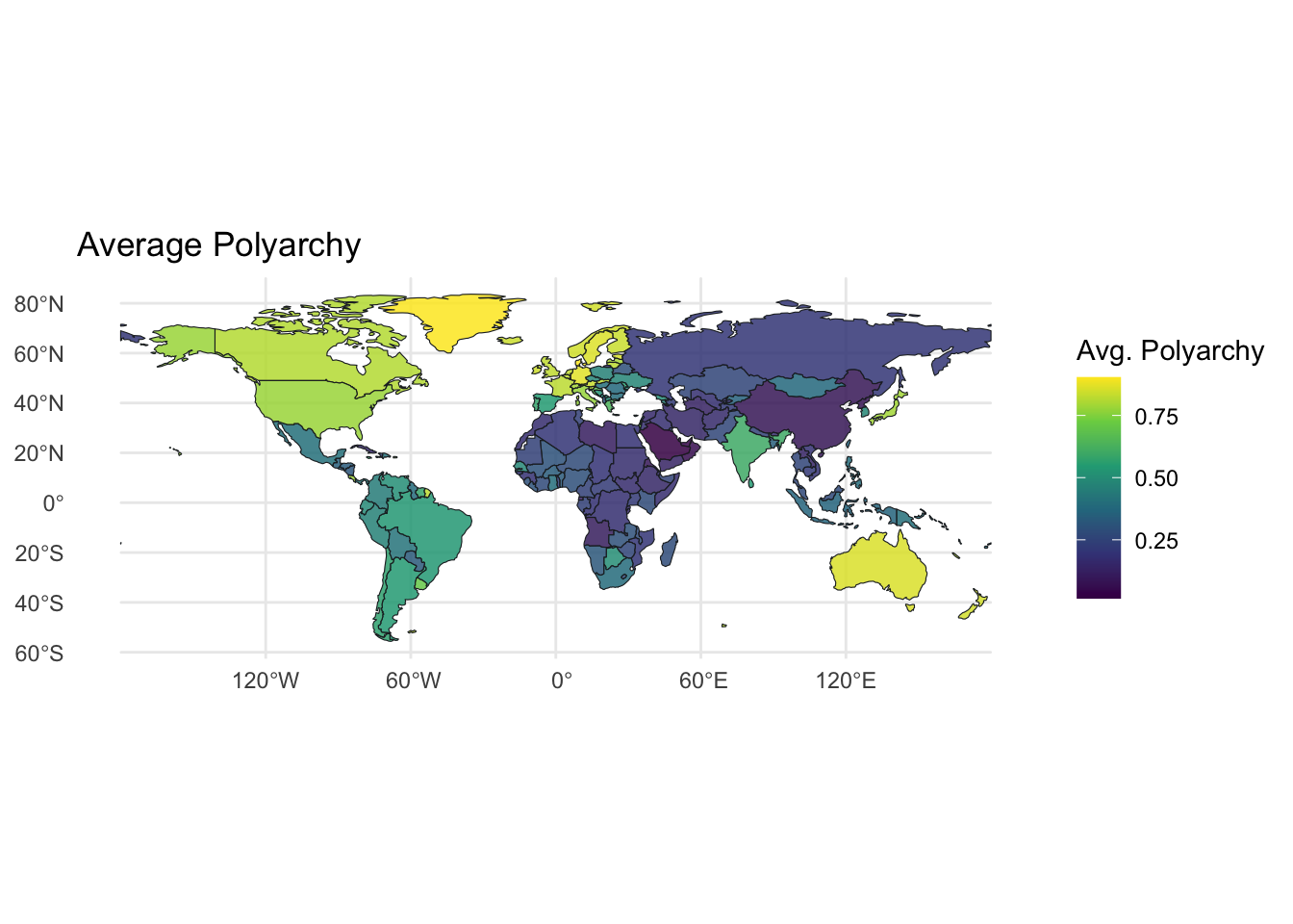
VDem
How’s that done?
library(vdemdata)
vdemdata::vdem -> vdem

vdem_map <- left_join(worldmap, vdem, by = c("SOVEREIGNT"="country_name"))
vdem_map %>%
  filter(year %in% c(1945:2023)) %>%
  filter(SOVEREIGNT != "Antarctica") %>%
  group_by(SOVEREIGNT, geometry) %>%
  summarise(avg_polyarchy = mean(v2x_polyarchy, na.rm = TRUE)) %>%
  ungroup() %>%
  ggplot() +
  geom_sf(aes(geometry = geometry, fill = avg_polyarchy),
          position = "identity", color = "#212529", linewidth = 0.2, alpha = 0.85) +
  scale_fill_viridis_c() +
  labs(fill="Avg. Polyarchy", title="Average Polyarchy") +
  theme_minimal()
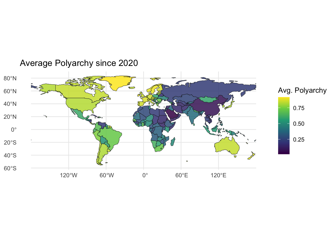
How’s that done?
vdem_map %>%
  filter(year %in% c(2020:2023)) %>%
  filter(SOVEREIGNT != "Antarctica") %>%
  group_by(SOVEREIGNT, geometry) %>%
  summarise(avg_polyarchy = mean(v2x_polyarchy, na.rm = TRUE)) %>%
  ungroup() %>%
  ggplot() +
  geom_sf(aes(geometry = geometry, fill = avg_polyarchy),
          position = "identity", color = "#212529", linewidth = 0.2, alpha = 0.85) +
  scale_fill_viridis_c() +
  labs(fill="Avg. Polyarchy", title="Average Polyarchy since 2020") +
  theme_minimal()
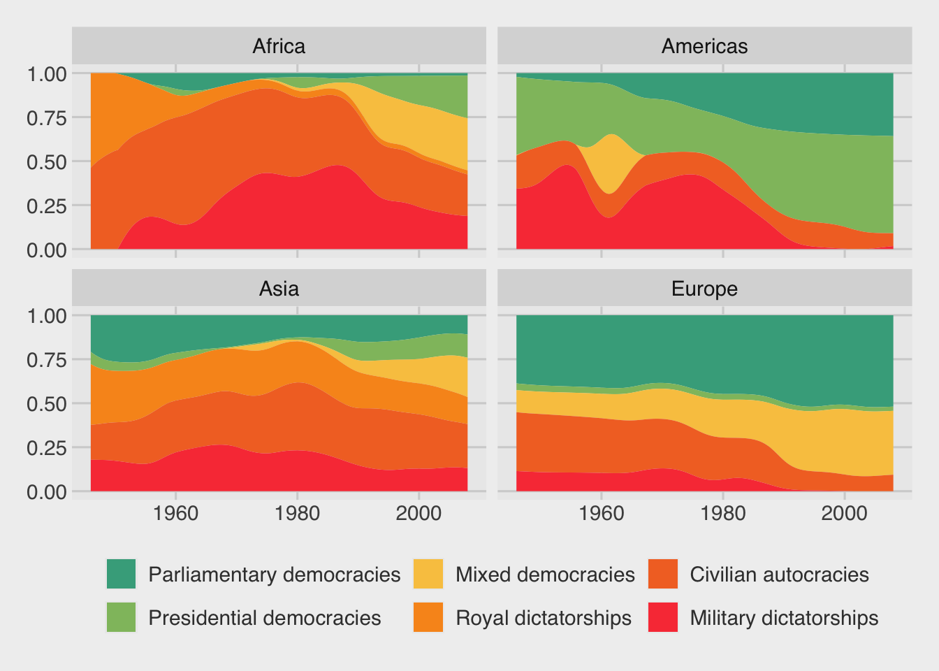
Democracy data
How’s that done?
library(democracyData)
library(tidyverse)
library(magrittr)       # for pipes
library(ggstream)       # proportion plots
library(ggthemes)       # nice ggplot themes
library(forcats)        # reorder factor variables
library(ggflags)        # add flags
library(peacesciencer)  # more great polisci data
library(countrycode)    # add ISO codes to countries
library(gganimate)

pacl %<>%
  mutate(regime_name = ifelse(regime == 0, "Parliamentary democracies",
       ifelse(regime == 1, "Mixed democracies",
       ifelse(regime == 2, "Presidential democracies",
       ifelse(regime == 3, "Civilian autocracies",
       ifelse(regime == 4, "Military dictatorships",
       ifelse(regime ==  5,"Royal dictatorships", regime))))))) %>%
  mutate(regime = as.factor(regime))

regime_palette <- c("Military dictatorships" = "#f94144",
                    "Civilian autocracies" = "#f3722c",
                    "Royal dictatorships" =  "#f8961e",
                    "Mixed democracies" = "#f9c74f",
                    "Presidential democracies" = "#90be6d",
                    "Parliamentary democracies" = "#43aa8b")
pacl %>%
  mutate(regime_name = as.factor(regime_name)) %>%
  mutate(regime_name = fct_relevel(regime_name, "Parliamentary democracies", "Presidential democracies", "Mixed democracies", "Royal dictatorships", "Civilian autocracies", "Military dictatorships")) %>%
  group_by(year, un_continent_name) %>%
  filter(!is.na(regime_name)) %>%
  count(regime_name) %>%
  ungroup() %>%
  filter(un_continent_name != "") %>%
  filter(un_continent_name != "Oceania") -> pacl_count

pacl_count %>%
    ggplot(aes(x = year, y = n,
               groups = regime_name,
               fill = regime_name)) +
    ggstream::geom_stream(type = "proportion") +
    facet_wrap(~un_continent_name) +
    scale_fill_manual(values = regime_palette) +
    ggthemes::theme_fivethirtyeight() +
    theme(legend.title = element_blank(),
          text = element_text(size = 14))
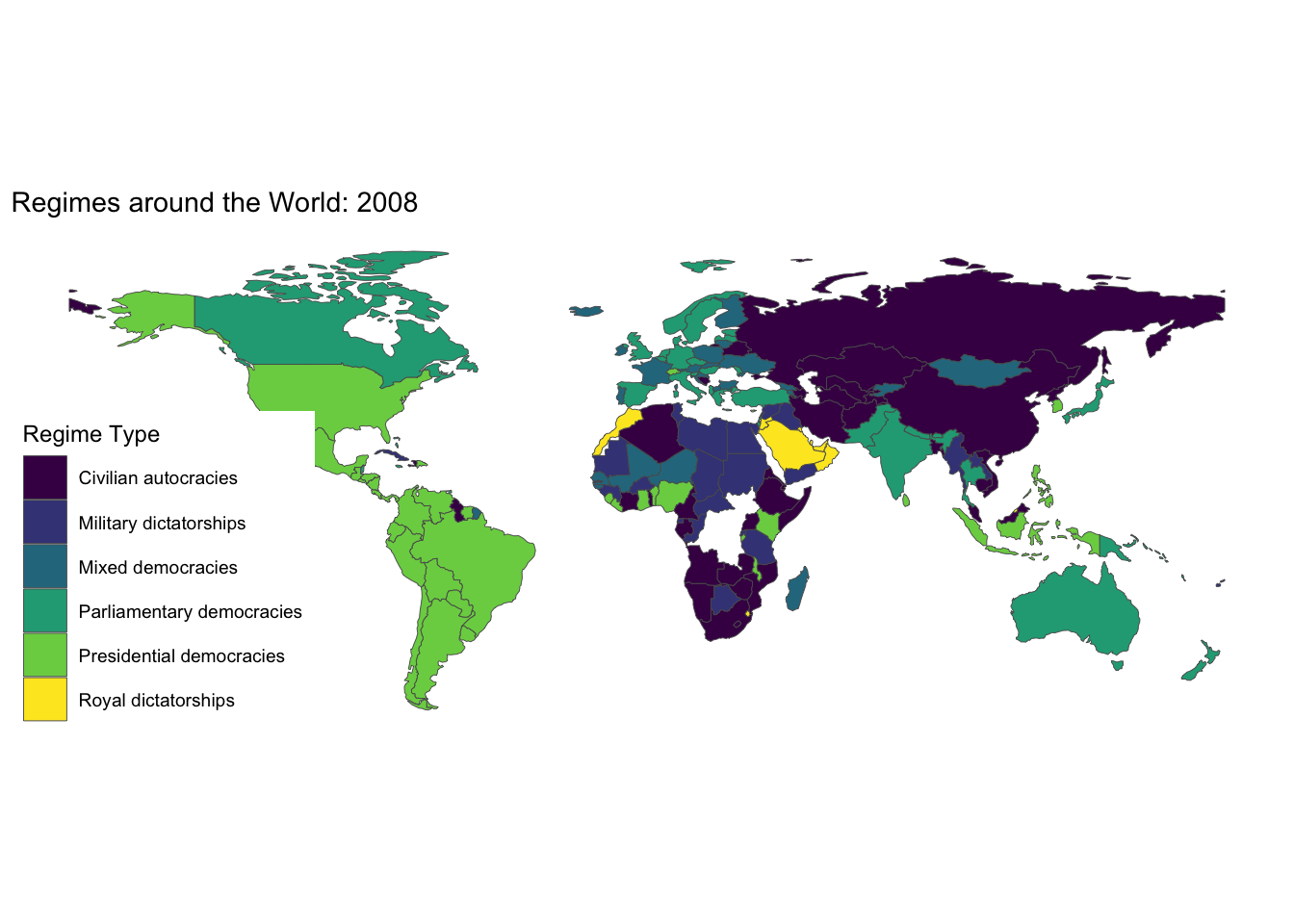
Regimes
How’s that done?
pacl_map <- left_join(worldmap, pacl, by=c("ADM0_A3" = "wdicode"))
animate.me <- pacl_map %>%  ggplot() + aes(fill=regime_name) + geom_sf(szie=0.1) + scale_fill_viridis_d()+ theme_map() + labs(title="Regimes around the World  - {closest_state}", fill="Regime Type") + transition_states(year)
animate.me
How’s that done?
pacl_map %>% filter(year==2008) %>% ggplot() + aes(fill=regime_name) + geom_sf(szie=0.1) + scale_fill_viridis_d()+ theme_map() + labs(title="Regimes around the World: 2008", fill="Regime Type")