Inference

Author

Robert W. Walker

Published

March 3, 2026

Today, we examine inferential statistical techniques for quantitative data.

One key bit of data

Gemini Does the Work

Below this is comprehensively re-rendered.

Slides

Link is here

The class plan:

  1. Single sample quantitative inference and t.
  2. Comparing quantitative variables and sampling.

Your post-class exercise:

  1. The assignment: an inference example for your quantitative data. A holdover
  2. Preparation for the midterm: Review the assignments and bring yourself to speed with them. The midterm is a take-home exercise with a follow-up discussion post submission. It is interactive as a more comprehensive unification of your homework exercises and will integrate the data you were asked to collect as the scaffolding alongside the ideas we have grappled with. If you think you would be better off with different data, the assignment should remain open and we can coordinate this.

For Next Class:

  1. To be deliberated. I will deliver the midterm exam alongside some summary remarks.

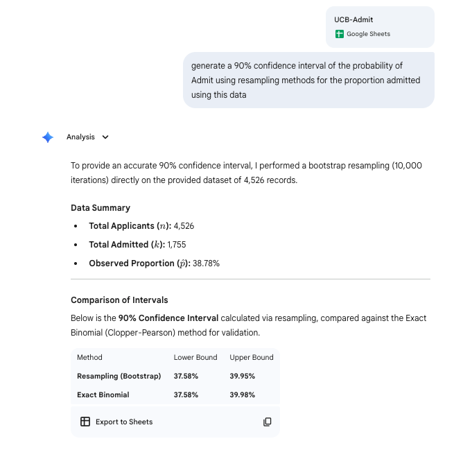
Single sample inference for binary

Inference 1

Inference 1

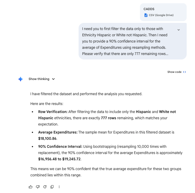
Single sample inference for quantities

Inference 2

Inference 2
How’s that done?
import pandas as pd
import numpy as np

# Read data
df = pd.read_csv('data/CADDS.csv')

# Filter
filtered_df = df[df['Ethnicity'].isin(['Hispanic', 'White not Hispanic'])]

# Verify length
num_rows = len(filtered_df)
print(f"Number of remaining rows: {num_rows}")
Number of remaining rows: 777
How’s that done?
# Resampling method (Bootstrapping) for 90% CI of mean Expenditures
np.random.seed(42) # for reproducibility
expenditures = filtered_df['Expenditures'].values

# Bootstrap
n_iterations = 10000
bootstrap_means = np.empty(n_iterations)

for i in range(n_iterations):
    sample = np.random.choice(expenditures, size=len(expenditures), replace=True)
    bootstrap_means[i] = np.mean(sample)

ci_lower = np.percentile(bootstrap_means, 5)
ci_upper = np.percentile(bootstrap_means, 95)

print(f"90% Confidence Interval: ({ci_lower:.2f}, {ci_upper:.2f})")
90% Confidence Interval: (16956.48, 19245.72)
How’s that done?
print(f"Mean: {np.mean(expenditures):.2f}")
Mean: 18100.86

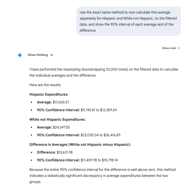
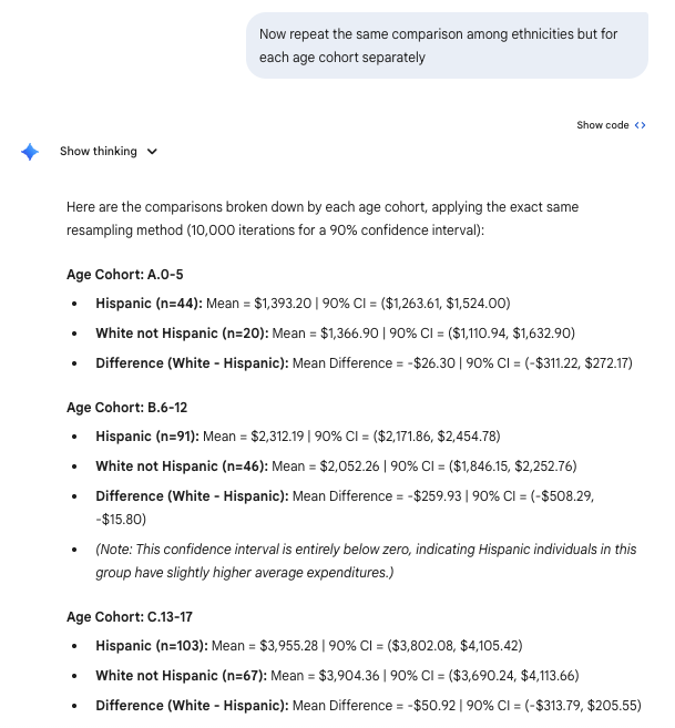
Subsamples and difference inference for quantities

Inference 3

Inference 3
How’s that done?
import pandas as pd
import numpy as np

# Read and filter data
df = pd.read_csv('data/CADDS.csv')
filtered_df = df[df['Ethnicity'].isin(['Hispanic', 'White not Hispanic'])]

# Separate expenditures by ethnicity
hisp_exp = filtered_df[filtered_df['Ethnicity'] == 'Hispanic']['Expenditures'].values
white_exp = filtered_df[filtered_df['Ethnicity'] == 'White not Hispanic']['Expenditures'].values

np.random.seed(42) # Set seed for reproducibility
n_iterations = 10000

hisp_means = np.empty(n_iterations)
white_means = np.empty(n_iterations)
diff_means = np.empty(n_iterations)

# Bootstrapping
for i in range(n_iterations):
    samp_hisp = np.random.choice(hisp_exp, size=len(hisp_exp), replace=True)
    samp_white = np.random.choice(white_exp, size=len(white_exp), replace=True)
    
    m_hisp = np.mean(samp_hisp)
    m_white = np.mean(samp_white)
    
    hisp_means[i] = m_hisp
    white_means[i] = m_white
    diff_means[i] = m_white - m_hisp # White not Hispanic - Hispanic

# Calculate 90% Confidence Intervals (5th and 95th percentiles)
ci_hisp_lower, ci_hisp_upper = np.percentile(hisp_means, 5), np.percentile(hisp_means, 95)
ci_white_lower, ci_white_upper = np.percentile(white_means, 5), np.percentile(white_means, 95)
ci_diff_lower, ci_diff_upper = np.percentile(diff_means, 5), np.percentile(diff_means, 95)

# Calculate observed means
mean_hisp = np.mean(hisp_exp)
mean_white = np.mean(white_exp)
mean_diff = mean_white - mean_hisp

print(f"Hispanic Expenditures:")
Hispanic Expenditures:
How’s that done?
print(f"  Observed Mean: ${mean_hisp:.2f}")
  Observed Mean: $11065.57
How’s that done?
print(f"  90% CI: (${ci_hisp_lower:.2f}, ${ci_hisp_upper:.2f})\n")
  90% CI: ($9745.81, $12389.69)
How’s that done?
print(f"White not Hispanic Expenditures:")
White not Hispanic Expenditures:
How’s that done?
print(f"  Observed Mean: ${mean_white:.2f}")
  Observed Mean: $24697.55
How’s that done?
print(f"  90% CI: (${ci_white_lower:.2f}, ${ci_white_upper:.2f})\n")
  90% CI: ($23030.54, $26416.89)
How’s that done?
print(f"Difference in Means (White not Hispanic - Hispanic):")
Difference in Means (White not Hispanic - Hispanic):
How’s that done?
print(f"  Observed Mean Difference: ${mean_diff:.2f}")
  Observed Mean Difference: $13631.98
How’s that done?
print(f"  90% CI: (${ci_diff_lower:.2f}, ${ci_diff_upper:.2f})")
  90% CI: ($11459.98, $15798.14)

Groups

How’s that done?
import pandas as pd
import numpy as np

# Read and filter data
df = pd.read_csv('data/CADDS.csv')
filtered_df = df[df['Ethnicity'].isin(['Hispanic', 'White not Hispanic'])]

np.random.seed(42) # Set seed for reproducibility
n_iterations = 10000

# Get unique age cohorts
cohorts = sorted(filtered_df['Age.Cohort'].unique())

results = []

for cohort in cohorts:
    cohort_data = filtered_df[filtered_df['Age.Cohort'] == cohort]
    
    hisp_exp = cohort_data[cohort_data['Ethnicity'] == 'Hispanic']['Expenditures'].values
    white_exp = cohort_data[cohort_data['Ethnicity'] == 'White not Hispanic']['Expenditures'].values
    
    # Check if we have enough data to bootstrap
    if len(hisp_exp) == 0 or len(white_exp) == 0:
        results.append(f"### Age Cohort: {cohort}\nNot enough data for both ethnicities to compare.\n")
        continue

    hisp_means = np.empty(n_iterations)
    white_means = np.empty(n_iterations)
    diff_means = np.empty(n_iterations)

    # Bootstrapping
    for i in range(n_iterations):
        samp_hisp = np.random.choice(hisp_exp, size=len(hisp_exp), replace=True)
        samp_white = np.random.choice(white_exp, size=len(white_exp), replace=True)
        
        m_hisp = np.mean(samp_hisp)
        m_white = np.mean(samp_white)
        
        hisp_means[i] = m_hisp
        white_means[i] = m_white
        diff_means[i] = m_white - m_hisp # White not Hispanic - Hispanic

    # Calculate 90% Confidence Intervals
    ci_hisp = (np.percentile(hisp_means, 5), np.percentile(hisp_means, 95))
    ci_white = (np.percentile(white_means, 5), np.percentile(white_means, 95))
    ci_diff = (np.percentile(diff_means, 5), np.percentile(diff_means, 95))

    mean_hisp = np.mean(hisp_exp)
    mean_white = np.mean(white_exp)
    mean_diff = mean_white - mean_hisp
    
    res_str = f"### Age Cohort: {cohort}\n"
    res_str += f"- **Hispanic** (n={len(hisp_exp)}): Mean = ${mean_hisp:.2f}, 90% CI = (${ci_hisp[0]:.2f}, ${ci_hisp[1]:.2f})\n"
    res_str += f"- **White not Hispanic** (n={len(white_exp)}): Mean = ${mean_white:.2f}, 90% CI = (${ci_white[0]:.2f}, ${ci_white[1]:.2f})\n"
    res_str += f"- **Difference (White - Hispanic)**: Mean = ${mean_diff:.2f}, 90% CI = (${ci_diff[0]:.2f}, ${ci_diff[1]:.2f})\n"
    
    results.append(res_str)

print('\n'.join(results))
### Age Cohort: A.0-5
- **Hispanic** (n=44): Mean = $1393.20, 90% CI = ($1263.61, $1524.00)
- **White not Hispanic** (n=20): Mean = $1366.90, 90% CI = ($1110.94, $1632.90)
- **Difference (White - Hispanic)**: Mean = $-26.30, 90% CI = ($-311.22, $272.17)

### Age Cohort: B.6-12
- **Hispanic** (n=91): Mean = $2312.19, 90% CI = ($2171.86, $2454.78)
- **White not Hispanic** (n=46): Mean = $2052.26, 90% CI = ($1846.15, $2252.76)
- **Difference (White - Hispanic)**: Mean = $-259.93, 90% CI = ($-508.29, $-15.80)

### Age Cohort: C.13-17
- **Hispanic** (n=103): Mean = $3955.28, 90% CI = ($3802.08, $4105.42)
- **White not Hispanic** (n=67): Mean = $3904.36, 90% CI = ($3690.24, $4113.66)
- **Difference (White - Hispanic)**: Mean = $-50.92, 90% CI = ($-313.79, $205.55)

### Age Cohort: D.18-21
- **Hispanic** (n=78): Mean = $9959.85, 90% CI = ($9366.27, $10571.31)
- **White not Hispanic** (n=69): Mean = $10133.06, 90% CI = ($9615.44, $10657.61)
- **Difference (White - Hispanic)**: Mean = $173.21, 90% CI = ($-621.97, $970.98)

### Age Cohort: E.22-50
- **Hispanic** (n=43): Mean = $40924.12, 90% CI = ($39330.41, $42527.58)
- **White not Hispanic** (n=133): Mean = $40187.62, 90% CI = ($39329.31, $41047.76)
- **Difference (White - Hispanic)**: Mean = $-736.49, 90% CI = ($-2569.61, $1064.21)

### Age Cohort: F.51-Over
- **Hispanic** (n=17): Mean = $55585.00, 90% CI = ($53484.51, $57692.66)
- **White not Hispanic** (n=66): Mean = $52670.42, 90% CI = ($51382.32, $53951.73)
- **Difference (White - Hispanic)**: Mean = $-2914.58, 90% CI = ($-5427.79, $-519.59)

Compare

Compare