How’s that done?
load(url("https://github.com/robertwwalker/DADMStuff/raw/master/Big-Week-6-RSpace.RData"))Linking Probability and Data
load(url("https://github.com/robertwwalker/DADMStuff/raw/master/Big-Week-6-RSpace.RData"))What is the probability of being admitted to UC Berkeley Graduate School?1
. . .
I have three variables:
Admitted or not
Gender
The department an applicant applied to.
Admission is the key.
library(janitor) #<<
UCBTab <- data.frame(UCBAdmissions) %>% reshape::untable(., .$Freq) %>% select(-Freq)
UCBTab %>% tabyl(Admit)  # Could also use UCBTab %$% table(Admit)
Admit n percent
Admitted 1755 0.3877596
Rejected 2771 0.6122404The proportion is denoted as \(\hat{p}\). We can also do this with table.
UCBTab %>% DT::datatable(.,fillContainer = FALSE, options = list(pageLength = 8), rownames=FALSE)library(viridisLite)
UCBTab %>% ggplot(.) + aes(x = Gender, fill = Admit) + geom_bar() + scale_fill_viridis_d()
Suppose we want to know \(\pi(Admit)\) – the probability of being admitted – with 90% probability.
We want to take the data that we saw and use it to infer the likely values of \(\pi(Admit)\).
Resampling/Simulation
Exact binomial computation
A normal approximation
Suppose I have 4526 chips with 1755 green and 2771 red.
. . .
I toss them all on the floor
. . .
and pick them up, one at a time,
. . .
record the value (green/red),
. . .
put the chip back,
[NB: I put it back to avoid getting exactly the same sample every time.]
. . .
and repeat 4526 times.
Each count of green chips as a proportion of 4526 total chips constitutes an estimate of the probability of Admit.
. . .
I wrote a little program to do just this – ResampleProps.
remotes::install_github("robertwwalker/ResampleProps")library(ResampleProps)
RSMP <- ResampleProp(UCBTab$Admit, k = 10000, tab.col = 1) %>% data.frame(Pi.Admit=., Gender=as.character("All"), frameN = 1)
quantile(RSMP$Pi.Admit, probs = c(0.05,0.95)) 5% 95%
0.3758285 0.3996907 What is our estimate of \(\pi\) with 90% confidence?
The probability of admission ranges from 0.376 to 0.4.
library(ggthemes)
RSMP %>%  ggplot(., aes(x=Pi.Admit)) + geom_density(outline.type = "upper", color="maroon") +labs(x=expression(pi)) + theme_minimal()
That last procedure is correct but it is overkill.
With probability of 0.05, how small could \(\pi\) be to have gotten 1755 of 4526 or more?
With probability 0.95, how big could \(\pi\) be to have gotten fewer than 1755 of 4526?
UCBTab %$% table(Admit) #<<Admit
Admitted Rejected
1755 2771 . . .
This is the exact binomial test.
UCBTab %$% table(Admit) %>% binom.test(conf.level = 0.9)
    Exact binomial test

data:  .
number of successes = 1755, number of trials = 4526, p-value < 2.2e-16
alternative hypothesis: true probability of success is not equal to 0.5
90 percent confidence interval:
 0.3757924 0.3998340
sample estimates:
probability of success
0.3877596 Plot.Me <- binom.test(1755, 1755+2771, conf.level=0.9)$conf.int %>% data.frame()With 90% probability, now often referred to as 90% confidence to avoid using the word probability twice, the probability of being admitted ranges between 0.3758 and 0.3998.
UCBTab %$% table(Admit) %>% binom.test(conf.level = 0.9)
    Exact binomial test

data:  .
number of successes = 1755, number of trials = 4526, p-value < 2.2e-16
alternative hypothesis: true probability of success is not equal to 0.5
90 percent confidence interval:
 0.3757924 0.3998340
sample estimates:
probability of success
0.3877596 c(pbinom(1755, 1755+2771, 0.3998340), pbinom(1754, 1755+2771, 0.3757924))[1] 0.05000037 0.95000004Binomial.Search <- data.frame(x=seq(0.33,0.43, by=0.001)) %>% mutate(Too.Low = pbinom(1755, 1755+2771, x), Too.High = 1-pbinom(1754, 1755+2771, x))
Binomial.Search %>% pivot_longer(cols=c(Too.Low,Too.High)) %>% ggplot(., aes(x=x, y=value, color=name)) + geom_line() + geom_hline(aes(yintercept=0.05)) + geom_hline(aes(yintercept=0.95)) + geom_vline(data=Plot.Me, aes(xintercept=.), linetype=3) + labs(title="Using the Binomial to Search", color="Greater/Lesser", x=expression(pi), y="Probability")
As long as \(n\) and \(\pi\) are sufficiently large, we can approximate this with a normal distribution. This will also prove handy for a related reason.
As long as \(n*\pi\) > 10, we can write that a standard normal \(z\) describes the distribution of \(\pi\), given \(n\) – the sample size and \(\hat{p}\) – the proportion of yes’s/true’s in the sample.
\[ Pr(\pi) = \hat{p} \pm z \cdot \left( \sqrt{\frac{\hat{p}*(1-\hat{p})}{n}} \right) \]
\(R\) implements this in prop.test. By default, R implements a modified version that corrects for discreteness/continuity. To get the above formula exactly, prop.test(table, correct=FALSE).
\[ z = \frac{\hat{p} - \pi}{\sqrt{\frac{\pi(1-\pi)}{n}}} \]
With some proportion calculated from data \(\hat{p}\) and some claim about \(\pi\) – hereafter called an hypothesis – we can use \(z\) to calculate/evaluate the claim. These claims are hypothetical values of \(\pi\). They can be evaluated against a specific alternative considered in three ways:
two-sided, that is \(\pi = value\) against not equal.
\(\pi \geq value\) against something smaller.
\(\pi \leq value\) against something greater.
In the first case, either much bigger or much smaller values could be evidence against equal. The second and third cases are always about smaller and bigger; they are one-sided.
Just as \(z\) has metric standard deviations now referred to as standard errors of the proportion, the z here will measure where the data fall with respect to the hypothetical \(\pi\).
With z sufficiently large, and in the proper direction, our hypothetical \(\pi\) becomes unlikely given the evidence and should be dismissed.
( Z.ALL <- (0.3877596 - 0.5)/(sqrt(0.5^2 / 4526)) ) # Calculate z [1] -15.10207The estimate is 15.1 standard errors below the hypothesized value.
\(\pi = 0.5\) against \(\pi \neq 0.5\).
pnorm(-abs(Z.ALL)) + (1-pnorm(abs(Z.ALL))) [1] 7.846435e-52Any \(|z| > 1.64\) – probability 0.05 above and below – is sufficient to dispense with the hypothesis.
\(\pi \leq 0.5\) against \(\pi \gt 0.5\).
With 90% confidence, \(z > 1.28\) is sufficient.
\(\pi \geq 0.5\) against \(\pi \lt 0.5\).
With 90% confidence, \(z < -1.28\) is sufficient.
prop.test(table(UCBTab$Admit), conf.level = 0.9, correct=FALSE)
    1-sample proportions test without continuity correction

data:  table(UCBTab$Admit), null probability 0.5
X-squared = 228.07, df = 1, p-value < 2.2e-16
alternative hypothesis: true p is not equal to 0.5
90 percent confidence interval:
 0.3759173 0.3997361
sample estimates:
        p
0.3877596
\(R\) reports the result as \(z^2\) not \(z\) which is \(\chi^2\) not normal; we can obtain the \(z\) by taking a square root: \[\sqrt{228.08} \approx 15.1 \]
This approximation yields an estimate of \(\pi\), with 90% confidence, that ranges between 0.376 and 0.4.
The formal equation defines:
\[ z = \frac{\hat{p} - \pi}{\sqrt{\frac{\pi(1-\pi)}{n}}} \]
Some language:
Margin of error is \(\hat{p} - \pi\). [MOE]
Confidence: the probability coverage given z [two-sided].
We need a guess at the true \(\pi\) because variance/std. dev. depend on \(\pi\). 0.5 is common because it maximizes the variance; we will have enough no matter what the true value.
Algebra allows us to solve for \(n\).
\[ n = \frac{z^2 \cdot \pi(1-\pi)}{(\hat{p} - \pi)^2} \]
Estimate the probability of supporting an initiative to within 0.03 with 95% confidence. Assume that the probability is 0.5 [it maximizes the variance and renders a conservative estimate – an upper bound on the sample size]
Sample.Size <- function(MOE, B.pi=0.5, Conf.lev=0.95) {
  My.n <- ((qnorm((1-Conf.lev)/2)^2)*(B.pi*(1-B.pi))) / MOE^2
  Necessary.sample <- ceiling(My.n)
  return(Necessary.sample)
}
Sample.Size(MOE=0.03, B.pi=0.5, Conf.lev = 0.95)
[1] 1068I need 1068 people to estimate support to within plus or minus 0.03 with 95% confidence.
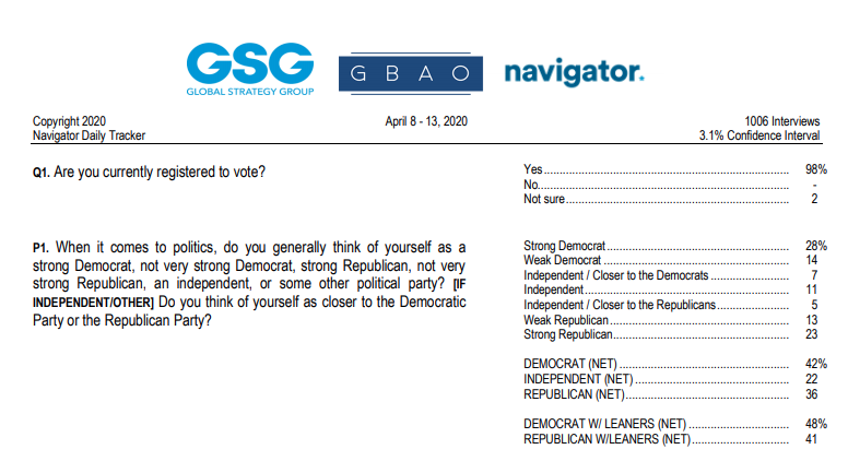
A real poll. They do not have quite enough for a 3% margin of error. But 1006 is enough for a 3.1 percent margin of error…
Sample.Size(MOE=0.031, B.pi=0.5, Conf.lev = 0.95)[1] 1000What is our estimate of \(\pi\) with 90% confidence?
The probability of admission ranges from 0.3758285 to 0.3996907.
If we wish to express this using the normal approximation, a central interval is the observed proportion plus/minus \(z\) times the standard error of the proportion – \[ SE(\hat{p}) = \sqrt{\frac{\hat{p}(1-\hat{p})}{n}} \] NB: The sample value replaces our assumed true value because \(\pi\) is to be solved for. For 90%, the probability of admissions ranges from
0.3877596 + qnorm(c(0.05,0.95))*(sqrt(0.3877596*(1-0.3877596)/4526))[1] 0.3758468 0.3996724Does the probability of admission depend on whether the applicant is Male or Female?
library(janitor); UCBTab %>% tabyl(Gender,Admit) %>% adorn_totals("col") Gender Admitted Rejected Total
Male 1198 1493 2691
Female 557 1278 1835UCBTab %>% tabyl(Gender,Admit) %>% adorn_percentages("row") Gender Admitted Rejected
Male 0.4451877 0.5548123
Female 0.3035422 0.6964578UCBTF <- UCBTab %>% filter(Gender=="Female")
UCBTF.Pi <- ResampleProp(UCBTF$Admit, k = 10000) %>% data.frame(Pi.Admit=., Gender=as.character("Female"), frameN=2) # Estimates for females
UCBTM <- UCBTab %>% filter(Gender=="Male")
UCBTM.Pi <- ResampleProp(UCBTM$Admit, k = 10000) %>% data.frame(Pi.Admit=., Gender = as.character("Male"), frameN = 2) # Estimates for malesUCBTM %$% table(Admit) %>% binom.test(., conf.level = 0.9)
    Exact binomial test

data:  .
number of successes = 1198, number of trials = 2691, p-value =
0.00000001403
alternative hypothesis: true probability of success is not equal to 0.5
90 percent confidence interval:
 0.4292930 0.4611706
sample estimates:
probability of success
             0.4451877
The probability of being admitted, conditional on being Male, ranges from 0.43 to 0.46 with 90% confidence.
UCBTM.Pi %>% ggplot(., aes(x=Pi.Admit)) + geom_density(color="maroon") + labs(x=expression(pi))
UCBTF %$% table(Admit) %>% binom.test(., conf.level = 0.9)
    Exact binomial test

data:  .
number of successes = 557, number of trials = 1835, p-value < 2.2e-16
alternative hypothesis: true probability of success is not equal to 0.5
90 percent confidence interval:
 0.2858562 0.3216944
sample estimates:
probability of success
             0.3035422
The probability of being of Admitted, given a Female, ranges from 0.286 to 0.322 with 90% confidence.
UCBTF.Pi %>% ggplot(., aes(x=Pi.Admit)) + geom_density(color="maroon") + labs(x=expression(pi))
Female: from 0.286 to 0.322
Male: from 0.43 to 0.46
All: from 0.3758 to 0.3998

UCB.Pi <- bind_rows(UCBTF.Pi, UCBTM.Pi)
UCB.Pi %>% ggplot(., aes(x=Gender, y=Pi.Admit, fill=Gender)) + geom_violin() + geom_label(aes(x=1.5, y=0.375), label="Too small to be male \n Too large to be female?", size=14, fill="black", color="white", inherit.aes = FALSE) + guides(size="none") + labs(x="") + scale_fill_viridis_d()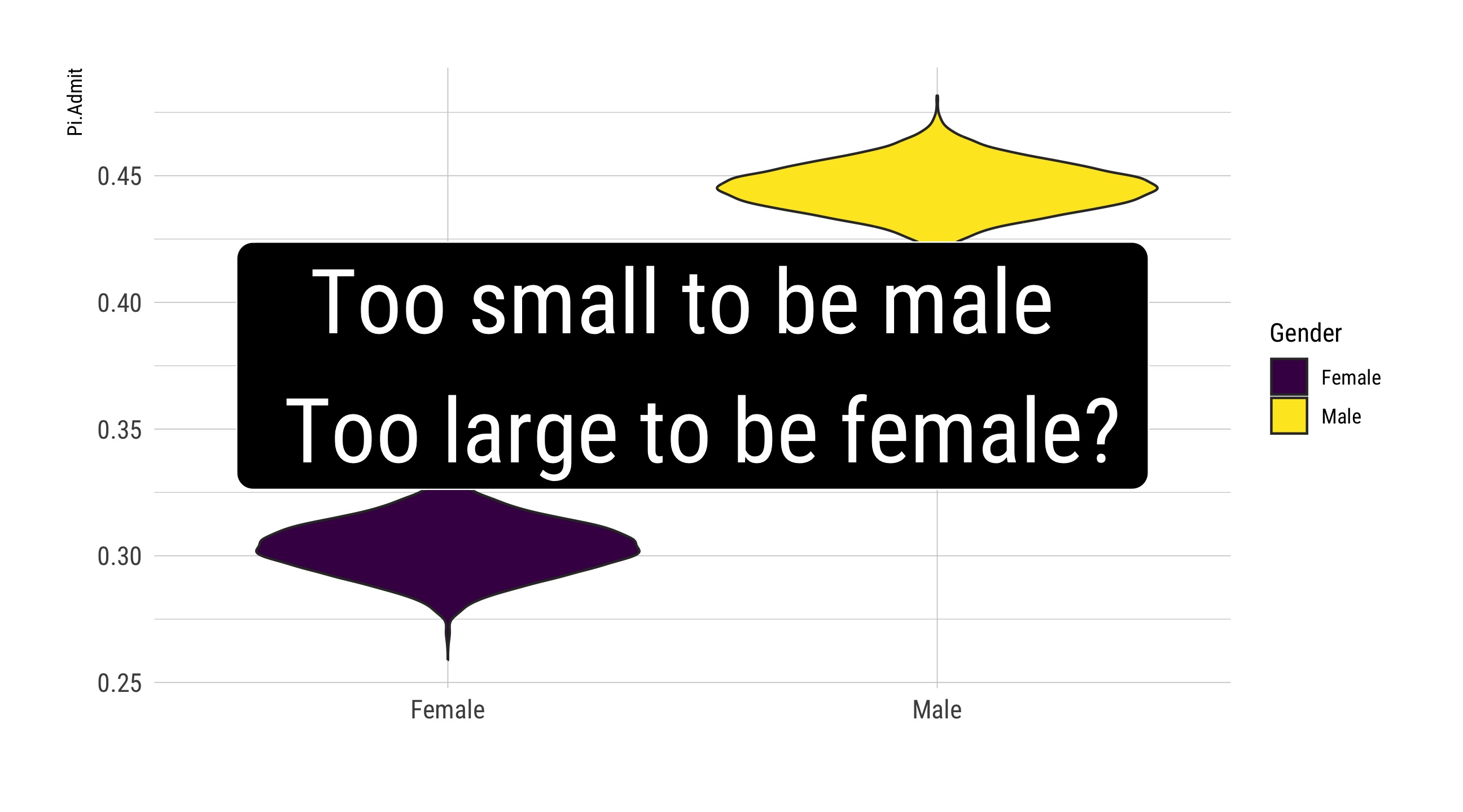
UCB.Pi <- bind_rows(UCBTF.Pi, UCBTM.Pi, RSMP)
UCB.Pi %>% ggplot(., aes(x=Pi.Admit, fill=Gender)) + geom_density(alpha=0.5) + theme_minimal() +  scale_fill_viridis_d() + transition_states(frameN, state_length = 40, transition_length = 20) + enter_fade() + exit_fade() -> SaveAnim
anim_save(SaveAnim, renderer = gifski_renderer(height=500, width=1000), filename="img/Anim1.gif")
How much more likely are Males to be admitted when compared to Females?
We can take the difference in our estimates for Male and Female.
UCB.Diff <- UCB.Pi %>% filter(frameN != 1) %>% select(Pi.Admit, Gender) %>% mutate(obs = rep(seq(1:10000),2)) %>% pivot_wider(., id_cols = obs, values_from=Pi.Admit, names_from=Gender) %>% mutate(Diff = Male - Female)
quantile(UCB.Diff$Diff, probs=c(0.05,0.95))
5% 95%
0.1176662 0.1651037 ggplot(UCB.Diff) + aes(x=Diff) + geom_density() + labs(title="Difference in Probability of Admission", subtitle="[Male - Female]")
\[[\hat{p}_{M} - \hat{p}_{F}] \pm z*\sqrt{ \underbrace{\frac{\hat{p}_{M}(1-\hat{p}_{M})}{n_{M}}}_{Males} + \underbrace{\frac{\hat{p}_{F}(1-\hat{p}_{F})}{n_{F}}}_{Females}}\]
# prop.test(table(UCBTab$Gender,UCBTab$Admit), conf.level=0.9, correct=FALSE)
UCBTab %$% table(Gender, Admit) %>% prop.test(conf.level = 0.9, correct=FALSE)
    2-sample test for equality of proportions without continuity correction

data:  .
X-squared = 92.205, df = 1, p-value < 2.2e-16
alternative hypothesis: two.sided
90 percent confidence interval:
 0.1179805 0.1653103
sample estimates:
   prop 1    prop 2
0.4451877 0.3035422
With 90% confidence, a Female is 0.118 to 0.165 [0.1416] less likely to be admitted.
Following something akin to the FOIL method, we can show that the variance of a difference in two random variables is the sum of the variances minus twice the covariance between them.
\[Var(X - Y) = Var(X) + Var(Y) - 2*Cov(X,Y) \]
If we assume [or recognize it is generally unknownable] that the male and female samples are independent, the covariance is zero, and the variance of the difference is simply the sum of the variance for male and female, respectively, and zero covariance.
\[SE(\hat{p}_{M} - \hat{p}_{F}) = \sqrt{ \underbrace{\frac{\hat{p}_{M}(1-\hat{p}_{M})}{n_{M}}}_{Males} + \underbrace{\frac{\hat{p}_{F}(1-\hat{p}_{F})}{n_{F}}}_{Females}}\]
The sum of \(k\) squared standard normal (z or Normal(0,1)) variates has a \(\chi^2\) distribution with \(k\) degrees of freedom. Two sample tests of proportions can be reported using the chi-square metric as well. \(R\)’s prop.test does this by default.
Of two forms:
. . .
We will now turn to the latter.
The central limit theorem – or, more aptly, central limit theorems – demonstrates that the sample mean is normally distributed under some – varying – set of conditions.
library(radiant)
result <- clt(dist = "Uniform", m = 1000)
plot(result, stat = "mean", bins = 50)
Exponential
result <- clt(dist = "Exponential", m = 1000, expo_rate = 4)
plot(result, stat = "mean", bins = 50)
What is the average level of expenditure by Ethnicity?
Why do we focus on the average? Under general conditions, the average has a known probability distribution even if the distribution of the underlying data is unknown. This is a result of the central limit theorem and a generic property of averaging. We can derive this distribution, it is known as \(t\) and has one parameter: degrees of freedom.
t distributionResults from the combination of a normal random variable in the numerator and a \(\chi^2\) random variable in the denominator. Both should generically hold from the central limit theorem.
Student’s \(t\) distribution generically describes the distribution of the difference between a sample mean and the true mean.
It has one parameter, the degrees of freedom.
First, a look at the data on expenditures.
load(url("https://github.com/robertwwalker/DADMStuff/raw/master/DiscriminationCADSS.RData"))
## Cutting Discrimination$Age into Discrimination$Age.Cohort
Discrimination$Age.Cohort <- cut(Discrimination$Age, include.lowest=FALSE,  right=TRUE,
                                 breaks=c(0, 5, 12, 17, 21, 50, 95))
WH <- Discrimination %>% filter(Ethnicity %in% c("White not Hispanic","Hispanic"))
datatable(WH)( BasePlot <- ggplot(WH, aes(x=Expenditures)) + geom_density(color="red") + theme_minimal() + labs(y="") )
library(crosstalk)
library(plotly)
shared_WH <- crosstalk::SharedData$new(WH)
Plot1 <- ggplot(shared_WH, aes(x=Ethnicity, y=Expenditures, color=Ethnicity)) + geom_jitter() + theme_minimal() + labs(y="")
p2 <- ggplotly(Plot1)
bscols(widths=c(1,11,12), "", list(
  filter_checkbox("Ethnicity", "Ethnicity", shared_WH, ~Ethnicity, inline=TRUE),
  filter_checkbox("Age.Cohort", "Age.Cohort", shared_WH, ~Age.Cohort, inline=TRUE),
  p2
))Suppose I have 777 chips that each contain an expenditure
. . .
I toss them all on the floor
. . .
and pick them up, one at a time,
. . .
record the value,
. . .
put the chip back,
[NB: I put it back to avoid getting exactly the same sample every time.]
. . .
and repeat this to create a sample of n=777.
. . .
Use random sampling to sample the mean/average 10000 times.
. . .
Each average of 777 chips/expenditures constitutes an estimate of the average expenditure.
WH.Means <- data.frame(Mean.Expenditure=ResampleMean(WH$Expenditures))( ggplot(WH, aes(x=Expenditures)) + geom_density() + theme_ipsum_rc() ) / (ggplot(WH.Means, aes(x=Mean.Expenditure)) + theme_ipsum_rc() ) + geom_density() + theme_ipsum_rc() 
What is the middle 90% of the sampled averages?
( ResQ <- quantile(WH.Means$Mean.Expenditure, probs=c(0.05,0.95)) ) 5% 95%
16853.97 19261.88 ResQD <- data.frame(ResQ=ResQ, Height2=5e-5)
BasePlot + geom_area(data=ResQD, aes(x=ResQ, y=Height2), fill="blue", color="blue", alpha=0.2, outline.type = "full")
Under general conditions, the sample and population mean can be described by the \(t_{df}\) distribution with a single parameter – degrees of freedom [df] – and metric standard errors of the mean: \(\frac{s}{\sqrt{n}}\) as follows:
\[ t_{df} = \frac{\overline{x} - \mu}{\frac{s}{\sqrt{n}}} \]
Given any observed sample of data, only two features of the aforementioned equation remain unknown: \(\mu\) – the true mean – and \(t_{df}\). Solving for \(\mu\) yields:
\[ \mu = \overline{x} - t_{df} \cdot \left( \frac{s}{\sqrt{n}} \right) \]
( Summaries <- WH %>% summarise(Exp.Mean = mean(Expenditures), Exp.SD = sd(Expenditures), Count = n()) ) Exp.Mean Exp.SD Count
1 18100.86 19579.53 777WH %$% t.test(Expenditures, conf.level = 0.9) #<<
    One Sample t-test

data:  Expenditures
t = 25.77, df = 776, p-value < 2.2e-16
alternative hypothesis: true mean is not equal to 0
90 percent confidence interval:
 16944.12 19257.61
sample estimates:
mean of x
 18100.86
With 90% confidence, average expenditures [for White not Hispanic and Hispanic] range between 16944 and 19258 dollars per DDS client.
ggplot(WH, aes(x=Ethnicity, y=Expenditures, fill=Ethnicity)) + geom_violin() + theme_ipsum_rc()
WH %>%
  filter(Ethnicity=="White not Hispanic") %$%
  t.test(Expenditures, conf.level=0.9)
    One Sample t-test

data:  Expenditures
t = 24.003, df = 400, p-value < 2.2e-16
alternative hypothesis: true mean is not equal to 0
90 percent confidence interval:
 23001.17 26393.92
sample estimates:
mean of x
24697.55 WH %>%
filter(Ethnicity=="Hispanic") %$%
t.test(Expenditures, conf.level=0.9)
    One Sample t-test

data:  Expenditures
t = 13.728, df = 375, p-value < 2.2e-16
alternative hypothesis: true mean is not equal to 0
90 percent confidence interval:
  9736.455 12394.683
sample estimates:
mean of x
11065.57 There are two [generic] ways to compare means:
1. The resampling approach
2. t-tests
The method is similar to the approach for comparing proportions. We will:
1. Take a random sample of the same size as the original for each group with replacement.
2. Calculate the average for each group and the difference in the averages.
3. Repeat steps 1 and 2 \(k\) times for \(k\) samples.
WNHExp <- Discrimination %>% filter(Ethnicity %in% c("White not Hispanic"))
HExp <- Discrimination %>% filter(Ethnicity %in% c("Hispanic"))
Expenditure.Difference <- data.frame(Diff=ResampleProps::ResampleDiffMeans(WNHExp$Expenditures,HExp$Expenditures))
Expenditure.Difference %>% ggplot(., aes(x=Diff)) + geom_density() + theme_minimal() + labs(x="Average Difference in Average White and Hispanic Expenditures")
t-testFor independent samples, the Behrens-Fisher problem dictates that comparisons of means have implications for the variance that must be reconciled. In short, we must assume that the variance and standard deviation of the samples are either the same [t] or different [Welch – the default].
In Welch’s case, the standard error is given by:
\[s_{\overline{x_{1}} - \overline{x_{2}}} = \sqrt{\frac{s^{2}_{1}}{n_{1}} + \frac{s^{2}_{2}}{n_{2}}}\] though the degrees of freedom follow a formula that involves the kurtosis of the samples [\(s^{4}\)].
Discrimination %>% filter(Ethnicity %in% c("White not Hispanic","Hispanic")) %>% t.test(Expenditures~Ethnicity, data=., conf.lev=0.9)
    Welch Two Sample t-test

data:  Expenditures by Ethnicity
t = -10.429, df = 743.08, p-value < 2.2e-16
alternative hypothesis: true difference in means between group Hispanic and group White not Hispanic is not equal to 0
90 percent confidence interval:
 -15784.59 -11479.37
sample estimates:
          mean in group Hispanic mean in group White not Hispanic
11065.57 24697.55 Discrimination %>% filter(Ethnicity %in% c("White not Hispanic","Hispanic")) %>% t.test(Expenditures~Ethnicity, data=., conf.lev=0.9, var.equal=TRUE)
    Two Sample t-test

data:  Expenditures by Ethnicity
t = -10.339, df = 775, p-value < 2.2e-16
alternative hypothesis: true difference in means between group Hispanic and group White not Hispanic is not equal to 0
90 percent confidence interval:
 -15803.25 -11460.71
sample estimates:
          mean in group Hispanic mean in group White not Hispanic
11065.57 24697.55 The paired t-test is a single sample average applied to the measured difference. The key is knowing who is matched with whom and believing that there is at least some variation in both outcomes that depends on the unit in question.
There is a linguistic distinction; this is an average difference instead of the previous difference in averages. The language describes the order of operation. For the paired comparison, I must know what to subtract from what.
Take the example of Concrete.
Twelve distinct batches of concrete are subjected to an additive. Does the additive strengthen concrete?
Concrete %>% datatable()For each batch, we can calculate the difference between those with and without an additive. To do so, we need mutate. Let’s plot it.
Concrete <- Concrete %>% mutate(Difference = Additive - No.Add)
hist(Concrete$Difference)
Concrete.Diff <- data.frame(Sampled.Mean.Difference = ResampleMean(Concrete$Difference))
quantile(Concrete.Diff$Sampled.Mean.Difference, probs=c(0.025, 0.975))
2.5% 97.5%
54.16667 262.50000 Concrete.Diff %>% ggplot() + aes(x=Sampled.Mean.Difference) + geom_density() + theme_ipsum_rc()
t.test(Concrete$Difference)
    One Sample t-test

data:  Concrete$Difference
t = 2.8793, df = 11, p-value = 0.01499
alternative hypothesis: true mean is not equal to 0
95 percent confidence interval:
  37.29936 279.36730
sample estimates:
mean of x
 158.3333
With 95% confidence, the additive increases the average break-weight of the concrete by 37.3 to 279.4 pounds.
With proportions: If we claim a value of \(\pi\), then use it for the standard error. If not, use the data.
With quantities: If comparing them, are samples independent or dependent? All the relevant quantities are known [or assumed] functions of the data.
For differences, the magic number is nearly always zero – no difference.
For one proportion:
ResampleProps::ResampleProp(vec.data, k=1000, tab.col=1)binom.test(x, n, alternative="?", p=0.5, conf.level=0.95)prop.test(x, n, alternative="?", p=0.5, conf.level=0.95, correct=TRUE)For two proportions:
prop.test(x=c(10,20), n=c(50, 50), alternative="?", p=0.5, conf.level=0.95, correct=TRUE)For one mean:
ResampleMeans::ResampleMean(vec.data, k=1000)t.test(x, alternative="?", mu=0, conf.level=0.95)For two means:
ResampleDiffMeans(vec.1, vec.2, k=1000)
Two types:
t.test(x, y, alternative="?", mu=0, conf.level=0.95, paired=FALSE, var.equal=FALSE)t.test(x, y, alternative="?", mu=0, conf.level=0.95, paired=TRUE)```
Do we want an hypothesis test or a confidence interval?
Choose a level of confidence/significance/probability.
If hypothesis test, derive the relevant critical value by combining the reference distribution with the level of confidence/significance/probability. What value of \(z\) or \(t\) would be required to reject the hypothesis? If an confidence interval, how many standard errors from the mean are covered by the given level of probability.
If an hypothesis test, calculate the test statistic.
Compute the confidence interval or compare the test statistic to the relevant critical value.
We probably think this depends on a bunch of applicant specific features but we will put that to the side for now.↩︎