Today, we will spend extensive time revisiting the logic of hypothesis testing and apply it to relationships among two variables along with a backward looking exploration of existing tests.
Causation is at the heart of the highest order human reasoning. Doing so with data is an objective if not an end result of modern fascination with machine learning. Yet, these are age old philosophical questions and modern work at the intersection of data and causation is perhaps best exemplified in the work of Judea Pearl. His most recent work, The Book of Why, details a lifetime of investigating causes and causal models at the intersection of computing, philosophy, and statistics. Though wide ranging, his podcast with Lex Fridman is worth listening to. The excerpt on correlation and causation is very useful.
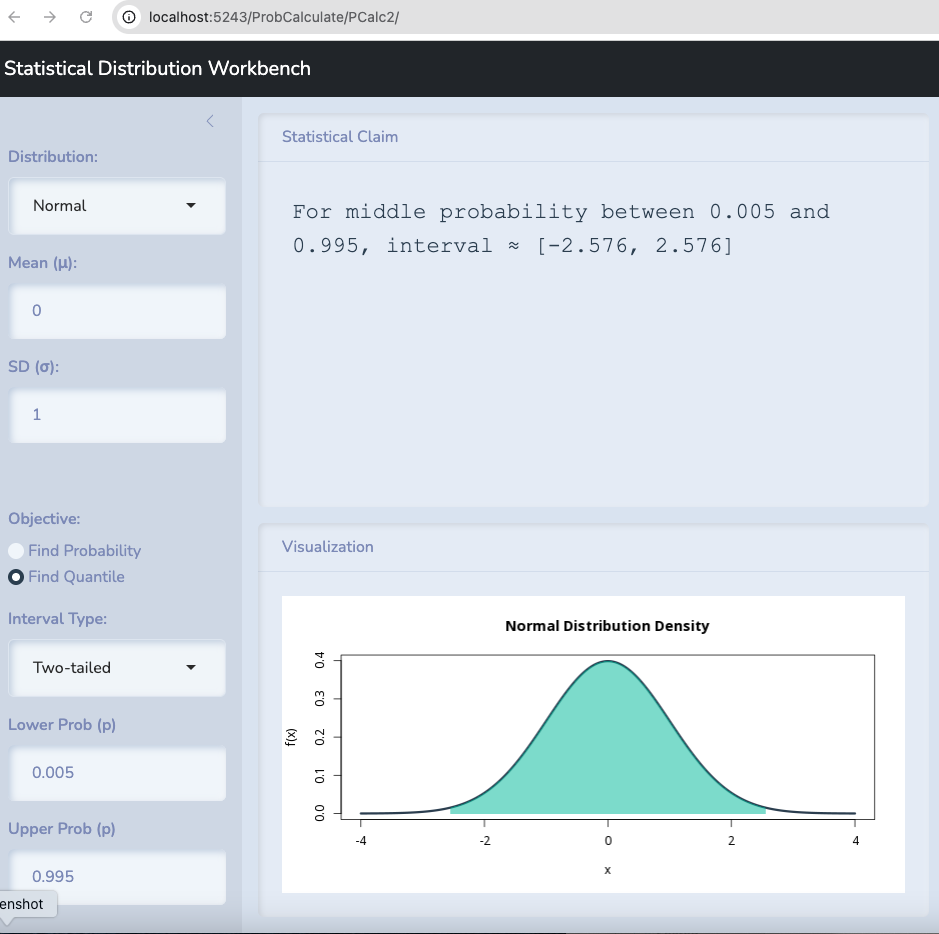
Let’s take the example of Berkeley. Let’s test the hypothesis that \(\pi=0.5\) first and let’s examine it with 99% confidence.
I will use the class tool to find that percentage.
Image
Anything within 2.576 standard deviations above or below the mean is possible with 99% confidence.
The standard error in this case is
\[\sqrt{\frac{\pi(1-\pi)}{n}}\]
This gives us \(0.5 \pm z*\) 0.0074321.
Or \(0.5 \pm 0.019\).
Anything between 0.481 and 0.519 could be observed if 0.5 is true.
A Single Tail
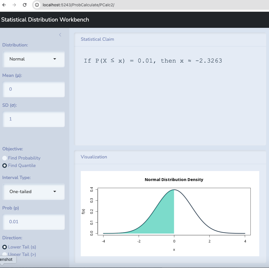
Let’s take the example of Berkeley. Let’s test the hypothesis that \(\pi \leq 0.5\) against the alternative that it is bigger and let’s examine it with 99% confidence.
I will use the class tool to find that percentage.
Image
Anything within 2.236 standard deviations above the mean is possible with 99% confidence.
The standard error in this case is
\[\sqrt{\frac{\pi(1-\pi)}{n}}\]
This gives us \(0.5 - z*\) 0.0074321.
Or \(0.5 + 2.236*0.019\).
Anything below 0.5166 could be observed if 0.5 or less is true.