Analytics I: Relationships among Data

Correlation and Hypotheses

Author

Robert W. Walker

Published

March 17, 2026

–

Summary Statistics are Insufficient

How’s that done?

load(url("https://github.com/robertwwalker/DADMStuff/raw/master/RegressionExamples.RData"))
datasaurus %>% group_by(dataset) %>% summarise(Mean.x = mean(x), Std.Dev.x = sd(x), Mean.y = mean(y), Std.Dev.y = sd(y)) %>% kable(format="html")

dataset	Mean.x	Std.Dev.x	Mean.y	Std.Dev.y
away	54.26610	16.76983	47.83472	26.93974
bullseye	54.26873	16.76924	47.83082	26.93573
circle	54.26732	16.76001	47.83772	26.93004
dino	54.26327	16.76514	47.83225	26.93540
dots	54.26030	16.76774	47.83983	26.93019
h_lines	54.26144	16.76590	47.83025	26.93988
high_lines	54.26881	16.76670	47.83545	26.94000
slant_down	54.26785	16.76676	47.83590	26.93610
slant_up	54.26588	16.76885	47.83150	26.93861
star	54.26734	16.76896	47.83955	26.93027
v_lines	54.26993	16.76996	47.83699	26.93768
wide_lines	54.26692	16.77000	47.83160	26.93790
x_shape	54.26015	16.76996	47.83972	26.93000

Relationships Matter

How’s that done?

datasaurus %>% ggplot() + aes(x=x, y=y, color=dataset) + geom_point() + guides(color=FALSE) + facet_wrap(vars(dataset))

A Deep Dive on Hypothesis Testing

A Proportions Example with the Normal

Revisiting Concrete

Always Visualize the Data

Models Use Inference to …

Unpack Black Boxes

We will literally do it with boxes/squares

Data and a Library

A Bit on Covariance and Correlation

Covariance is defined as: \[\sum_{i} (x_{i} - \overline{x})(y_{i} - \overline{y})\]

Where \(\overline{x}\) and \(\overline{y}\) are the sample means of x and y. The items in parentheses are deviations from the mean; covariance is the product of those deviations from the mean. The metric of covariance is the product of the metric of \(x\) and \(y\); often something for which no baseline exists. For this reason, we use a normalized form of covariance known as correlation, often just \(\rho\).

\[\rho_{xy} = \sum_{i} \frac{(x_{i} - \overline{x})(y_{i} - \overline{y})}{s_{x}s_{y}}\]

Correlation is a normed measure; it varies between -1 and 1.

An Oregon Gender Gap

A random sample of salaries in the 1990s for new hires from Oregon DAS. I know nothing about them. It is worth noting that these data represent a protected class by Oregon statute. We have a state file or we can load the data from github.

How’s that done?

OregonSalaries %>% 
  select(-Obs) %>% 
  mutate(Row = rep(c(1:16),2)) %>% 
  pivot_wider(names_from = Gender, values_from = Salary) %>% select(-Row)

# A tibble: 16 × 2
   Female   Male
    <dbl>  <dbl>
 1 41514. 47343.
 2 40964. 46382.
 3 39170. 45813.
 4 37937. 46410.
 5 33982. 43796.
 6 36077. 43124.
 7 39174. 49444.
 8 39037. 44806.
 9 29132. 44440.
10 36200. 46680.
11 38561. 47337.
12 33248. 47299.
13 33609. 41461.
14 33669. 43598.
15 37806. 43431.
16 35846. 49266.

   Obs   Salary Gender
1    1 41514.39 Female
2    2 40964.07 Female
3    3 39170.19 Female
4    4 37936.57 Female
5    5 33981.78 Female
6    6 36077.27 Female
7    7 39174.06 Female
8    8 39037.37 Female
9    9 29131.75 Female
10  10 36200.45 Female
11  11 38561.40 Female
12  12 33247.92 Female
13  13 33609.49 Female
14  14 33669.22 Female
15  15 37805.83 Female
16  16 35846.13 Female
17  17 47342.66   Male
18  18 46382.39   Male
19  19 45812.91   Male
20  20 46409.66   Male
21  21 43796.05   Male
22  22 43124.02   Male
23  23 49443.82   Male
24  24 44805.79   Male
25  25 44440.32   Male
26  26 46679.59   Male
27  27 47337.10   Male
28  28 47298.73   Male
29  29 41461.05   Male
30  30 43598.29   Male
31  31 43431.18   Male
32  32 49266.41   Male

Visualising Independent Samples

How’s that done?

ggplot(OregonSalaries) + aes(x=Gender, y=Salary) + geom_boxplot() + theme_xaringan()

Visualising Independent Samples

How’s that done?

ggplot(OregonSalaries) + aes(x=Gender, y=Salary, fill=Gender) + geom_violin() + theme_xaringan()

About Those Squares: Deviations

The mean of all salaries is 41142.433. Represented in equation form, we have:

\[Salary_{i} = \alpha + \epsilon_{i}\]

The \(i^{th}\) person’s salary is some average salary \(\alpha\) [or perhaps \(\mu\) to maintain conceptual continuity] (shown as a solid blue line) plus some idiosyncratic remainder or residual salary for individual \(i\) denoted by \(\epsilon_{i}\) (shown as a blue arrow). Everything here is measured in dollars.

\[Salary_{i} = 41142.433 + \epsilon_{i}\]

# A tibble: 16 × 2
   Female[,1] Male[,1]
        <dbl>    <dbl>
 1       372.    6200.
 2      -178.    5240.
 3     -1972.    4670.
 4     -3206.    5267.
 5     -7161.    2654.
 6     -5065.    1982.
 7     -1968.    8301.
 8     -2105.    3663.
 9    -12011.    3298.
10     -4942.    5537.
11     -2581.    6195.
12     -7895.    6156.
13     -7533.     319.
14     -7473.    2456.
15     -3337.    2289.
16     -5296.    8124.

. . .

By definition, those vertical distances would/will sum to zero. This sum to zero constraint is what consumes a degree of freedom; it is why the standard deviation has N-1 degrees of freedom. The distance from the point to the line is also shown in blue; that is the observed residual salary. It shows how far that individual’s salary is from the overall average.

Square Them

A Big Black Box

# A tibble: 16 × 2
   Female[,1]  Male[,1]
        <dbl>     <dbl>
 1    138350. 38442803.
 2     31813. 27457097.
 3   3889736. 21813358.
 4  10277545. 27743644.
 5  51274988.  7041698.
 6  25655866.  3926692.
 7   3874503. 68912991.
 8   4431282. 13420200.
 9 144256540. 10876058.
10  24423237. 30660131.
11   6661738. 38373872.
12  62323288. 37899934.
13  56745270.   101515.
14  55848872.  6031248.
15  11132919.  5238385.
16  28050778. 65999032.

  sum(Salary.Deviation.Squared)
1                     892955384

The Black Box of Salaries

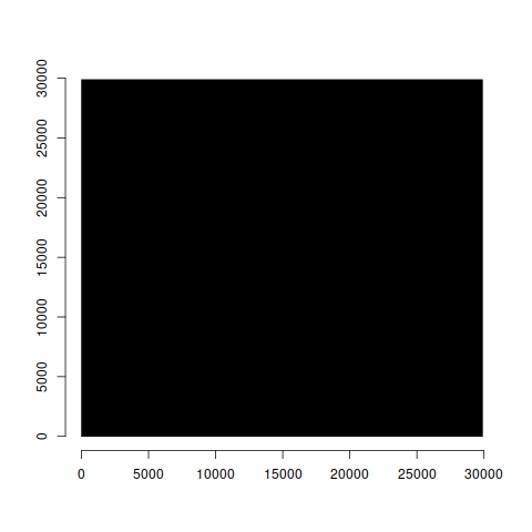
The total area of the black box in the original metric (squared dollars) is: 892955385. The length of each side is the square root of that area, e.g. 29882.36 in dollars.

This square, when averaged by degrees of freedom and called mean square, has a known distribution, \(\chi^2\) if we assume that the deviations, call them errors, are normal.

The \(\chi^2\) distribution

The \(\chi^2\) [chi-squared] distribution can be derived as the sum of \(k\) squared \(Z\) or standard normal variables. Because they are squares, they are always positive. The \(k\) is called degrees of freedom. Differences in \(\chi^2\) also have a \(\chi^2\) distribution with degrees of freedom equal to the difference in degrees of freedom.

As a technical matter (for x > 0): \[f(x) = \frac{1}{2^{\frac{k}{2}}\Gamma(k/2)} x^{\frac{k}{2-1}}e^{\frac{-x}{2}}\]

Some language and \(F\)

Sum of squares: \[\sum_{i=1}^{N} e_{i}^{2}\] Mean square: divide the sum of squares by \(k\) degrees of freedom. NB: Take the square root and you get the standard deviation. \[\frac{1}{k}\sum_{i=1}^{N} e_{i}^{2}\]

Fisher’s \(F\) ratio or the \(F\) describes the ratio of two \(\chi^2\) variables (mean square) with numerator and denominator degrees of freedom. It is the ratio of [degrees of freedom] averaged squared errors. As the ratio becomes large, we obtain greater evidence that the two are not the same. Let’s try that here.

The Core Conditional

But all of this stems from the presumption that \(e_{i}\) is normal; that is a claim that cannot really be proven or disproven. It is a core assumption that we should try to verify/falsify.

Because the \(e_{i}\) being normal means implies that their squares are \(\chi^2\)^a and further that the ratio of their mean-squares are \(F\).

As an aside, the technical definition of \(t\)^b is a normal divided by the square root of a \(\chi^2\) so \(t\) and \(F\) must be equivalent with one degree of freedom in the numerator.

^a This is why the various results in prop.test are reported as X-squared.

^b I mentioned this fact previously when introducing t (defined by degrees of freedom and with metric standard error.)

Verification of the Normal

Plots [shape]
the quantile-quantile plot
Statistical tests

plots

How’s that done?

plot(density(lm(OregonSalaries$Salary~1)$residuals), main="Residual Salary")

the quantile-quantile plot of a normal

The mean of residual salary is zero. The standard deviation is the root-mean-square. Compare observed residual salary [as z] to the hypothetical normal.

How’s that done?

data.frame(x=scale(lm(OregonSalaries$Salary~1)$residuals)) %>% arrange(x) %>%  mutate(y=qnorm(seq(1, length(OregonSalaries$Salary))/33)) %>% ggplot() + aes(x=x, y=y) + geom_point()

tests

We can examine the claim that residual salary is plausibly normal by examining the slope of the sample and theoretical quantiles: the slope of the q-q plot. This is exactly what the following does under the null hypothesis of a normal.

How’s that done?

shapiro.test(lm(Salary~1, data=OregonSalaries)$residuals)


    Shapiro-Wilk normality test

data:  lm(Salary ~ 1, data = OregonSalaries)$residuals
W = 0.9591, p-value = 0.2595

There are a few others. I personally prefer gvlma.

Linear Models

Will expand on the previous by unpacking the box, reducing residual squares via the inclusion of features, explanatory variables, explanatory factors, exogenous inputs, predictor variables. In this case, let us posit that salary is a function of gender. As an equation, that yields:

\[Salary_{i} = \alpha + \beta_{1}*Gender_{i} + \epsilon_{i}\] We want to measure that \(\beta\); in this case, the difference between Male and Female. By default, R will include Female as the constant.

What does the regression imply? That salary for each individual \(i\) is a function of a constant and gender. Given the way that R works, \(\alpha\) will represent the average for females and \(\beta\) will represent the difference between male and female average salaries. The \(\epsilon\) will capture the difference between the individual’s salary and the average of their group (the mean of males or females).

A New Residual Sum of Squares

The picture will now have a red line and a black line and the residual/leftover/unexplained salary is now the difference between the point and the respective vertical line (red arrows or black arrows). What is the relationship between the datum and the group mean? The answer is shown in black/red.

The Squares

The sum of the remaining squared vertical distances is 238621277 and is obtained by squaring each black/red number and summing them. The amount explained by gender [measured in squared dollars] is the difference between the sums of blue and black/red numbers, squared. It is important to notice that the highest paid females and the lowest paid males may have more residual salary given two averages but the different averages, overall, lead to far less residual salary than a single average for all salaries. Indeed, gender alone accounts for:

How’s that done?

sum(scale(OregonSalaries$Salary, scale = FALSE)^2) - sum(lm(Salary~Gender, data=OregonSalaries)$residuals^2)

[1] 654334108

Intuitively, Gender should account for 16 times the squared difference between Female and Overall Average (4522) and 16 times the squared difference between Male and Overall Average (4522).

How’s that done?

32*(mean(OregonSalaries$Salary[OregonSalaries$Gender=="Female"], na.rm=TRUE)-mean(OregonSalaries$Salary))^2

[1] 654334108

A Visual: What Proportion is Accounted For?

Regression Tables

How’s that done?

Model.1 <- lm(Salary~Gender, data=OregonSalaries)
summary(Model.1)


Call:
lm(formula = Salary ~ Gender, data = OregonSalaries)

Residuals:
    Min      1Q  Median      3Q     Max 
-7488.7 -2107.9   433.3  1743.9  4893.9 

Coefficients:
            Estimate Std. Error t value       Pr(>|t|)    
(Intercept)  36620.5      705.1   51.94        < 2e-16 ***
GenderMale    9043.9      997.1    9.07 0.000000000422 ***
---
Signif. codes:  0 '***' 0.001 '**' 0.01 '*' 0.05 '.' 0.1 ' ' 1

Residual standard error: 2820 on 30 degrees of freedom
Multiple R-squared:  0.7328,    Adjusted R-squared:  0.7239 
F-statistic: 82.26 on 1 and 30 DF,  p-value: 0.0000000004223

Analysis of Variance: The Squares

F is the ratio of the two mean squares. It is also \(t^2\).

.small[

How’s that done?

anova(Model.1)

Analysis of Variance Table

Response: Salary
          Df    Sum Sq   Mean Sq F value          Pr(>F)    
Gender     1 654334108 654334108  82.264 0.0000000004223 ***
Residuals 30 238621277   7954043                            
---
Signif. codes:  0 '***' 0.001 '**' 0.01 '*' 0.05 '.' 0.1 ' ' 1

]

The Idea Scales to both Quantitative Variables and Multiple Categories

A Multi-Category Example

How’s that done?

result <- radiant.model::regress(
  WH, 
  rvar = "Expenditures", 
  evar = "Age.Cohort"
)
summary(result, sum_check = c("rmse", "sumsquares", "confint"))

Linear regression (OLS)
Data     : WH 
Response variable    : Expenditures 
Explanatory variables: Age.Cohort 
Null hyp.: the effect of Age.Cohort on Expenditures is zero
Alt. hyp.: the effect of Age.Cohort on Expenditures is not zero

                  coefficient std.error t.value p.value    
 (Intercept)         2224.912   330.017   6.742  < .001 ***
 Age.Cohort|0 - 5    -839.928   584.850  -1.436   0.151    
 Age.Cohort|13-17    1710.299   443.488   3.856  < .001 ***
 Age.Cohort|18-21    7816.237   458.709  17.040  < .001 ***
 Age.Cohort|22-50   38142.650   440.101  86.668  < .001 ***
 Age.Cohort|51 +    51042.473   537.290  95.000  < .001 ***

Signif. codes:  0 '***' 0.001 '**' 0.01 '*' 0.05 '.' 0.1 ' ' 1

R-squared: 0.961,  Adjusted R-squared: 0.961 
F-statistic: 3833.317 df(5,771), p.value < .001
Nr obs: 777 

Prediction error (RMSE):  3847.81 
Residual st.dev   (RSD):  3862.753 

Sum of squares:
            df                  SS
Regression   5 285,981,965,641.547
Error      771  11,503,984,347.992
Total      776 297,485,949,989.540

                 coefficient      2.5%     97.5%      +/-
(Intercept)         2224.912  1577.073  2872.751  647.839
Age.Cohort|0 - 5    -839.928 -1988.016   308.160 1148.088
Age.Cohort|13-17    1710.299   839.713  2580.886  870.586
Age.Cohort|18-21    7816.237  6915.771  8716.704  900.467
Age.Cohort|22-50   38142.650 37278.711 39006.589  863.939
Age.Cohort|51 +    51042.473 49987.748 52097.198 1054.725

Not Alot Left….

How’s that done?

black.box.maker(result$model)

Bullseye

Messy

How’s that done?

qqnorm(residuals(result$model))

What about Ethnicity?

How’s that done?

Model.3 <- lm(Expenditures ~ Ethnicity + Age.Cohort, data=WH)
summary(Model.3)


Call:
lm(formula = Expenditures ~ Ethnicity + Age.Cohort, data = WH)

Residuals:
     Min       1Q   Median       3Q      Max 
-20075.0  -1206.7      0.1   1202.1  16446.7 

Coefficients:
                            Estimate Std. Error t value Pr(>|t|)    
(Intercept)                   2359.9      344.7   6.846 1.55e-11 ***
EthnicityWhite not Hispanic   -402.1      298.3  -1.348 0.178045    
Age.Cohort0 - 5               -849.3      584.6  -1.453 0.146685    
Age.Cohort13-17               1733.8      443.6   3.908 0.000101 ***
Age.Cohort18-21               7870.0      460.2  17.101  < 2e-16 ***
Age.Cohort22-50              38311.5      457.4  83.768  < 2e-16 ***
Age.Cohort51 +               51227.2      554.2  92.432  < 2e-16 ***
---
Signif. codes:  0 '***' 0.001 '**' 0.01 '*' 0.05 '.' 0.1 ' ' 1

Residual standard error: 3861 on 770 degrees of freedom
Multiple R-squared:  0.9614,    Adjusted R-squared:  0.9611 
F-statistic:  3198 on 6 and 770 DF,  p-value: < 2.2e-16

Confidence Intervals

How’s that done?

confint(Model.3)

                                 2.5 %     97.5 %
(Intercept)                  1683.2345  3036.6106
EthnicityWhite not Hispanic  -987.6405   183.4497
Age.Cohort0 - 5             -1996.8464   298.2797
Age.Cohort13-17               862.9646  2604.5597
Age.Cohort18-21              6966.5797  8773.3519
Age.Cohort22-50             37413.6880 39209.3043
Age.Cohort51 +              50139.2506 52315.1525

Comparison

How’s that done?

anova(result$model, Model.3)

Analysis of Variance Table

Model 1: Expenditures ~ Age.Cohort
Model 2: Expenditures ~ Ethnicity + Age.Cohort
  Res.Df         RSS Df Sum of Sq      F Pr(>F)
1    771 11503984348                           
2    770 11476899027  1  27085321 1.8172  0.178

At the margin, Ethnicity accounts for little variance.

Some Basic Cost Accounting

\[Total.Cost_{t} = \alpha + \beta*units_t + \epsilon_{t}\]

With data on per period (t) costs and units produced, we can partition fixed \(\alpha\) and variable costs \(\beta\) (or cost per unit). Consider the data on Handmade Bags. We want to accomplish two things. First, to measure the two key quantities. Second, be able to predict costs for hypothetical number of units.

A comment on correlation

The Data

How’s that done?

HMB %>% skim() %>% kable(format = "html", digits = 3)

skim_type	skim_variable	n_missing	complete_rate	numeric.mean	numeric.sd	numeric.p0	numeric.p25	numeric.p50	numeric.p75	numeric.p100	numeric.hist
numeric	units	0	1	351.967	131.665	141.00	241.5	356.00	457.0	580.00	▇▇▆▇▆
numeric	TotCost	0	1	19946.865	2985.202	14357.98	17593.8	20073.93	22415.2	24887.83	▆▇▇▇▇

A Look at the Data

How’s that done?

p1 <- ggplot(HMB) + aes(x=units, y=TotCost) + geom_point() + labs(y="Total Costs per period", x="Units")
plotly::ggplotly(p1)

The Thing to Measure

How’s that done?

p1 <- ggplot(HMB) + aes(x=units, y=TotCost) + geom_point() + geom_smooth(method="lm") + labs(y="Total Costs per period", x="Units")
plotly::ggplotly(p1)

A Linear Model

How’s that done?

Model.HMB <- lm(TotCost ~ units, data=HMB)
summary(Model.HMB)


Call:
lm(formula = TotCost ~ units, data = HMB)

Residuals:
    Min      1Q  Median      3Q     Max 
-1606.7  -610.9  -124.8   509.8  2522.3 

Coefficients:
             Estimate Std. Error t value Pr(>|t|)    
(Intercept) 12308.642    323.601   38.04   <2e-16 ***
units          21.702      0.862   25.18   <2e-16 ***
---
Signif. codes:  0 '***' 0.001 '**' 0.01 '*' 0.05 '.' 0.1 ' ' 1

Residual standard error: 871.8 on 58 degrees of freedom
Multiple R-squared:  0.9162,    Adjusted R-squared:  0.9147 
F-statistic: 633.8 on 1 and 58 DF,  p-value: < 2.2e-16

\[Total.Cost_{t} = 12308.64 + 21.70 * units_t + \epsilon_{t}\] where \(\epsilon_{t}\) has a standard deviation of 872 dollars.

`fitted.values()` or predictions

The line is the fitted values.

How’s that done?

data.frame(units=HMB$units, TotCost = HMB$TotCost, Fitted = fitted.values(Model.HMB)) %>% ggplot() + aes(x=units, y=TotCost) + geom_point() + geom_line(aes(x=units, y=Fitted)) + scale_x_continuous(limits=c(0,600)) + scale_y_continuous(limits=c(0,25000))

Residual Costs?

How’s that done?

data.frame(Residual.Cost = residuals(Model.HMB)) %>% ggplot() + aes(sample=Residual.Cost) + geom_qq() + geom_qq_line()

Not the Prettiest but the best….

How’s that done?

car::qqPlot(residuals(Model.HMB))

Because normal is sustainable, I can ….

Interpret the table including \(t\) and \(F\).
Utilize confidence intervals for the estimates.
Predict from the regression of two forms.
Subject to examinations of other characteristics of the regression.

`anova` [Sums of squares]

How’s that done?

anova(Model.HMB)

Analysis of Variance Table

Response: TotCost
          Df    Sum Sq   Mean Sq F value    Pr(>F)    
units      1 481694173 481694173  633.81 < 2.2e-16 ***
Residuals 58  44080089    760002                      
---
Signif. codes:  0 '***' 0.001 '**' 0.01 '*' 0.05 '.' 0.1 ' ' 1

Two types of squares: those a function of units and those residual. Why?

`confint` confidence intervals

From normal, the slope and intercept have \(t\) confidence intervals.

How’s that done?

confint(Model.HMB,level = 0.95)

                  2.5 %      97.5 %
(Intercept) 11660.88464 12956.39966
units          19.97605    23.42705

With 95% confidence, fixed costs range from 11660.88 to 12956.40 dollars per period and the variable costs range from 19.976 to 23.427 dollars per unit. If the goal is to attain 20 dollars per unit, we cannot rule that out [though a 95 percent lower bound would].

How’s that done?

confint(Model.HMB,level = 0.9)

                    5 %        95 %
(Intercept) 11767.72623 12849.55807
units          20.26066    23.14245

Plots

How’s that done?

RegressionPlots(Model.HMB)

Predicting Costs

Average Costs `interval="confidence"`

How’s that done?

predict(Model.HMB, newdata=data.frame(units=c(200,250,300)), interval="confidence")

       fit      lwr      upr
1 16648.95 16303.25 16994.66
2 17734.03 17448.18 18019.88
3 18819.11 18576.63 19061.58

All Costs `interval="prediction"`

How’s that done?

predict(Model.HMB, newdata=data.frame(units=c(200,250,300)), interval="prediction")

       fit      lwr      upr
1 16648.95 14869.98 18427.92
2 17734.03 15965.71 19502.35
3 18819.11 17057.28 20580.93

Diminshing Marginal Cost?

How’s that done?

Semiconductors %>% ggplot() + aes(x=units, y=TotCost4) + geom_point() + geom_smooth(method = "lm") + geom_smooth(method = "loess", color="red") + theme_xaringan() + labs(x="Units", y="Total Cost", title="Semiconductors")

Residuals

How’s that done?

SClm <- lm(TotCost4~units, data=Semiconductors)
SClm2 <- lm(TotCost4~poly(units, 2, raw=TRUE), data=Semiconductors)
par(mfrow=c(2,2))
plot(SClm)

Residuals

How’s that done?

resid.plotter(SClm2)

Comparing Squares

How’s that done?

anova(SClm,SClm2)

Analysis of Variance Table

Model 1: TotCost4 ~ units
Model 2: TotCost4 ~ poly(units, 2, raw = TRUE)
  Res.Df       RSS Df Sum of Sq     F      Pr(>F)    
1     58 304149603                                   
2     57 203027172  1 101122431 28.39 0.000001757 ***
---
Signif. codes:  0 '***' 0.001 '**' 0.01 '*' 0.05 '.' 0.1 ' ' 1

Lines?

How’s that done?

PPlm <- lm(TotCost3 ~ units:PlantFac, data=PowerPlant)
PowerPlant %>% ggplot() + aes(x=units, y=TotCost3, color=PlantFac) + geom_point() + geom_smooth(method = "lm") + theme_xaringan() + labs(x="Units", y="Total Cost", title="Power Plant")

Comparison

test or anova

How’s that done?

PPlm1 <- lm(TotCost3~units, data=PowerPlant)
PPlm2 <- lm(TotCost3~PlantFac*units, data=PowerPlant)
anova(PPlm1,PPlm)

Analysis of Variance Table

Model 1: TotCost3 ~ units
Model 2: TotCost3 ~ units:PlantFac
  Res.Df       RSS Df Sum of Sq      F       Pr(>F)    
1     58 585943761                                     
2     56 348638405  2 237305356 19.059 0.0000004859 ***
---
Signif. codes:  0 '***' 0.001 '**' 0.01 '*' 0.05 '.' 0.1 ' ' 1

How’s that done?

anova(PPlm,PPlm2)

Analysis of Variance Table

Model 1: TotCost3 ~ units:PlantFac
Model 2: TotCost3 ~ PlantFac * units
  Res.Df       RSS Df Sum of Sq      F Pr(>F)
1     56 348638405                           
2     54 345221354  2   3417052 0.2672 0.7665

The Premier League

How’s that done?

Model.EPL <- lm(Points ~ Wage.Bill.milGBP, data=EPL)
summary(Model.EPL)


Call:
lm(formula = Points ~ Wage.Bill.milGBP, data = EPL)

Residuals:
    Min      1Q  Median      3Q     Max 
-12.569  -3.201   0.353   3.712  11.129 

Coefficients:
                 Estimate Std. Error t value       Pr(>|t|)    
(Intercept)      32.11589    2.74905  11.683 0.000000000776 ***
Wage.Bill.milGBP  0.24023    0.02987   8.042 0.000000227415 ***
---
Signif. codes:  0 '***' 0.001 '**' 0.01 '*' 0.05 '.' 0.1 ' ' 1

Residual standard error: 6.438 on 18 degrees of freedom
Multiple R-squared:  0.7823,    Adjusted R-squared:  0.7702 
F-statistic: 64.67 on 1 and 18 DF,  p-value: 0.0000002274

\[Points = 32.12 + 0.24*Wage.Bill + \epsilon\]

How’s that done?

EPL$FV <- fitted.values(Model.EPL)
PP <- ggplot(EPL) + aes(x=Wage.Bill.milGBP, y=Points, text=Team) + geom_point() + geom_smooth(method="lm", color="black")
PP

How’s that done?

plotly::ggplotly(PP)

Not Unreasonable

How’s that done?

qqnorm(residuals(Model.EPL))

Residuals

How’s that done?

resid.plotter(Model.EPL)

Predicting Points

How’s that done?

head(predict(Model.EPL, newdata=data.frame(Wage.Bill.milGBP=seq(0,200,10)), interval = "confidence"), 10)

        fit      lwr      upr
1  32.11589 26.34036 37.89143
2  34.51820 29.26702 39.76939
3  36.92051 32.16859 41.67244
4  39.32282 35.03629 43.60936
5  41.72513 37.85788 45.59239
6  44.12744 40.61679 47.63809
7  46.52975 43.29225 49.76725
8  48.93206 45.86190 52.00222
9  51.33437 48.30814 54.36060
10 53.73668 50.62574 56.84762

Some Concluding Remarks

It’s all about squares. But really, it’s all about normals.
Assessing normality is crucial to inference in linear models. But we cannot really know whether or not it holds. But if it does:
1. Slopes and intercepts are t, as are their confidence intervals.
2. Sums of squares have ratios defined by F.
3. Predictions have t averages and normal intervals.
4. All founded upon the sum of squared errors being \(\chi^2\).
This core idea of explaining variance or unpacking a black box is the core question to virtually all machine learning and modelling.
The capital asset pricing model.

Other Formats

Summary Statistics are Insufficient

Relationships Matter

A Deep Dive on Hypothesis Testing

A Proportions Example with the Normal

Revisiting Concrete

Always Visualize the Data

Models Use Inference to …

Unpack Black Boxes

We will literally do it with boxes/squares

Data and a Library

A Bit on Covariance and Correlation

An Oregon Gender Gap

Visualising Independent Samples

Visualising Independent Samples

About Those Squares: Deviations

Square Them

A Big Black Box

The Black Box of Salaries

The \(\chi^2\) distribution

Some language and \(F\)

The Core Conditional

Verification of the Normal

plots

the quantile-quantile plot of a normal

tests

Linear Models

A New Residual Sum of Squares

The Squares

A Visual: What Proportion is Accounted For?

Regression Tables

Analysis of Variance: The Squares

The Idea Scales to both Quantitative Variables and Multiple Categories

A Multi-Category Example

Not Alot Left….

Bullseye

Messy

What about Ethnicity?

Confidence Intervals

Comparison

Some Basic Cost Accounting

The Data

A Look at the Data

The Thing to Measure

A Linear Model

fitted.values() or predictions

Residual Costs?

Not the Prettiest but the best….

Because normal is sustainable, I can ….

anova [Sums of squares]

confint confidence intervals

Plots

Predicting Costs

Average Costs interval="confidence"

All Costs interval="prediction"

Diminshing Marginal Cost?

Residuals

Residuals

Comparing Squares

Lines?

Comparison

The Premier League

Not Unreasonable

Residuals

Predicting Points

Some Concluding Remarks

`fitted.values()` or predictions

`anova` [Sums of squares]

`confint` confidence intervals

Average Costs `interval="confidence"`

All Costs `interval="prediction"`