Today, we will spend extensive time revisiting the logic of hypothesis testing and apply it to relationships among two variables along with a backward looking exploration of existing tests.

Two key bits of data

CADDS.
Berkeley.

Hypotheses must be complete

With binary data, all we have is $\pi$ or $\hat{p}$. Whichever we have, we use.

Slides

Link is here

The class plan:

Squares, correlation and regression
a Claude app

Your post-class exercise:

The midterm.
Use an LLM and the suggested materials to grapple with Pearl’s argument.

Hypothesis Testing

How’s that done?

Concrete <- read.csv("data/Concrete.csv")
Concrete

   Batch No.Add Additive Diff
1      1   4550     4600  -50
2      2   4950     4900   50
3      3   6250     6650 -400
4      4   5700     5950 -250
5      5   5350     5700 -350
6      6   5300     5400 -100
7      7   5150     5400 -250
8      8   5800     5850  -50
9      9   4900     4850   50
10    10   6050     6450 -400
11    11   5550     5850 -300
12    12   5750     5600  150

How’s that done?

mean(Concrete$Diff)

[1] -158.3333

How’s that done?

sd(Concrete$Diff)

[1] 190.4938

How’s that done?

sd(Concrete$Diff)/sqrt(12)

[1] 54.99082

How’s that done?

(mean(Concrete$Diff) - 0)/(sd(Concrete$Diff)/sqrt(12))

[1] -2.879269

On Causality

Causation is at the heart of the highest order human reasoning. Doing so with data is an objective if not an end result of modern fascination with machine learning. Yet, these are age old philosophical questions and modern work at the intersection of data and causation is perhaps best exemplified in the work of Judea Pearl. His most recent work, The Book of Why, details a lifetime of investigating causes and causal models at the intersection of computing, philosophy, and statistics. Though wide ranging, his podcast with Lex Fridman is worth listening to. The excerpt on correlation and causation is very useful.

He develops a ladder of causation. This is quite well explained in this two page primer.

Associational
Interventional
Counterfactual

We want to understand precisely how these various levels influence what we learn from data and deploy data to accomplish.

Judea Pearl’s website

The book on statistics and causal inference

A lecture on the Book of Why

Sections 2.1 to 2.10 of the Causal Mixtape are a very succinct read.

Illustrating an Hypothesis Test with the Normal

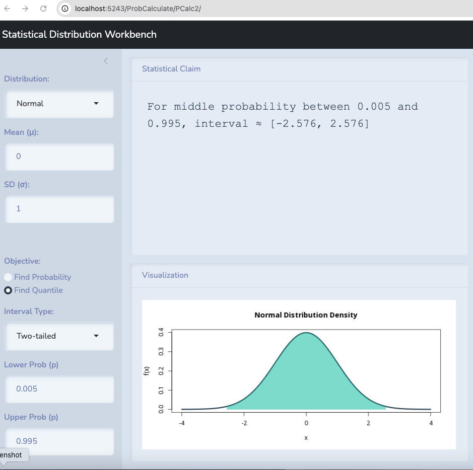
Let’s take the example of Berkeley. Let’s test the hypothesis that $\pi=0.5$ first and let’s examine it with 99% confidence.

I will use the class tool to find that percentage.

Anything within 2.576 standard deviations above or below the mean is possible with 99% confidence.

The standard error in this case is

\[\sqrt{\frac{\pi(1-\pi)}{n}}\]

This gives us $0.5 \pm z*$ 0.0074321.

Or $0.5 \pm 0.019$.

Anything between 0.481 and 0.519 could be observed if 0.5 is true.

A Single Tail

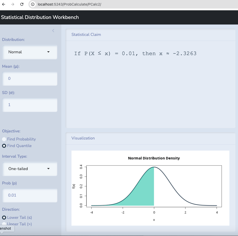
Let’s take the example of Berkeley. Let’s test the hypothesis that $\pi \leq 0.5$ against the alternative that it is bigger and let’s examine it with 99% confidence.

I will use the class tool to find that percentage.

Anything within 2.236 standard deviations above the mean is possible with 99% confidence.

The standard error in this case is

\[\sqrt{\frac{\pi(1-\pi)}{n}}\]

This gives us $0.5 - z*$ 0.0074321.

Or $0.5 + 2.236*0.019$.

Anything below 0.5166 could be observed if 0.5 or less is true.

Overview

This document illustrates how ordinary least squares (OLS) regression applies to cost accounting. We simulate 52 weeks of production data, estimate a cost function, and explore the regression output interactively.

The data-generating process (DGP) is:

\[\text{Cost}_t = \underbrace{16{,}750}_{\text{fixed overhead}} + \underbrace{150}_{\beta_1} \times \text{Units}_t + \underbrace{\varepsilon_t}_{\text{error}}\]

where $\varepsilon_t \sim \mathcal{N}(16{,}750,\; 4{,}000^2)$ and $\text{Units}_t$ follows a Poisson distribution with arrival rate $\lambda = 2{,}000$ truncated below at $1{,}500$.

Intercept interpretation

The error term has a non-zero mean of $16,750, so the effective DGP intercept is $16{,}750 + 16{,}750 = \$33{,}500$. The OLS estimator targets this combined value. Managers should distinguish the accounting fixed cost ($16,750) from the statistical intercept estimated by regression.

Parameters

Simulation parameters
Parameter	Symbol	Value
Poisson arrival rate	$\lambda$	2,000 units
Truncation lower bound	—	1,500 units
Variable cost per unit	$\beta_1$	$150
Fixed overhead	$\beta_0^{\text{acct}}$	$16,750
Error mean	$\mu_\varepsilon$	$16,750
Error std dev	$\sigma_\varepsilon$	$4,000
Effective DGP intercept	$\beta_0^{\text{DGP}}$	$33,500
Sample size	$n$	52 weeks

Interactive explorer

The widget below generates a fresh 52-week sample and provides four analytical views. Use the New sample button to resample and observe how estimates vary.

Observations

R²

—

Slope (β₁)

—

Intercept (β₀)

—

Show: OLS fit True DGP 95% CI band

X-axis:

Residual mean

—

Residual std dev

—

RMSE

—

Drag slider to set production volume and read off cost forecast.

Units: 2,000

OLS prediction

—

95% PI lower

—

95% PI upper

—

Decomposition

—

Conceptual notes

Scatter plot

Each point is one week. The OLS line minimises the sum of squared vertical distances from each point to the line. Key comparisons:

OLS fit vs True DGP — in practice the true line is never observed; this toggle shows how well estimation recovers it from one year of data.
95% CI band — confidence in the mean cost at a given volume level, narrowest near $\bar{x}$ and widening at the extremes.

Residuals diagnostic

What to look for

A well-specified model shows residuals randomly scattered around zero with constant spread. Systematic patterns suggest:

Fan shape — heteroskedasticity (variance grows with output)
Curve — non-linearity (a quadratic term may help)
Drift over time — an omitted seasonal or trend variable

Distributions

Distribution panel guide
Panel	What it shows
Units	Left boundary at 1,500 visible; Poisson shape above
Total costs	Driven by both volume variation and the error term
Residuals	Should look approximately bell-shaped, centred near zero

Prediction intervals

The 95% prediction interval (PI) is wider than a confidence interval (CI) because it covers a single future week, not the mean:

\[\hat{y} \pm t_{n-2,\,0.025} \cdot \hat{\sigma}\sqrt{1 + \frac{1}{n} + \frac{(x^* - \bar{x})^2}{\sum(x_i - \bar{x})^2}}\]

Key formula reference

Parameter truth vs. estimation
Component	True value	OLS target
Intercept $\beta_0$	$33,500	Varies by sample
Slope $\beta_1$	$150 / unit	Varies by sample
Error std dev $\sigma$	$4,000	RMSE $\approx$ $4,000

Sampling variability

Resample repeatedly to observe how much $\hat{\beta}_0$, $\hat{\beta}_1$, and $R^2$ fluctuate. Regression coefficients are themselves random variables.

Simulated data — not real company figures.