
Probability Distributions
Linking Probability and Data
A Bit on Trees and Juries
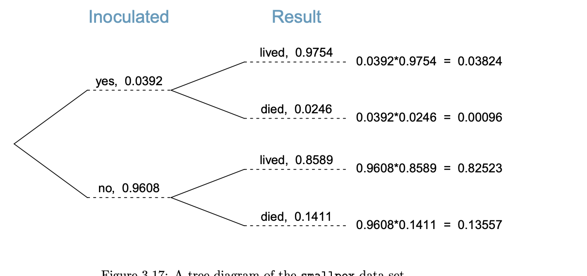
- P(Died|Inoculated): 0.0246.
- P(Lived|Inoculated): 0.9754.
- P(Died|Not Inoculated): 0.8589.
- P(Lived|Not Inoculated): 0.1411.
The computation on the right is the law of total probability.
- P(Died,Inoculated): 0.0392*0.0246=0.00096.
- P(Lived,Inoculated): 0.0392*0.9754=0.03824.
- P(Died,Not Inoculated): 0.9608*0.8589=0.82523.
- P(Lived,Not Inoculated): 0.9608*0.1411=0.13557.
Jurors
Three nodes: guilty and not at each, convict at the third.
The trick is (1) that evidence has to match or charges would be dropped and (2) we cannot escape the prior.
Jurors
Three nodes: guilty and not at each, convict at the third.
What are the chances of a random match?
- Blood type: P(NG|Match) = 0.45.
- Fingerprints: P(NG|Match) = 0.21.
- DNA: P(NG|Match) = 0.017.
\[ P(G|M,M,M) = \frac{P(G)*1*1*1}{P(G)*1*1*1 + (1-P(G))*0.45*0.21*0.017} \]
The Bayes Factor: A Ratio
\[ P(G|M,M,M) = \frac{P(G)*1*1*1}{P(G)*1*1*1 + (1-P(G))*0.45*0.21*0.017} \\ P(NG|M,M,M) = \frac{(1-P(G))*0.45*0.21*0.017}{P(G)*1*1*1 + (1-P(G))*0.45*0.21*0.017} \]
A Core Idea: Independence
What does it mean to say something is independent of something else?
- The simplest way to think about it is, “do I learn something more about x by knowing y than not”. If two things are independent, I don’t need to care about y if x is my objective.
It really struggles to spell/typeset in graphics
Representing Probability Distributions
Is of necessity two-dimensional,
- We have \(x\) and
- and \(Pr(X=x)\) in one of two types (Pr or f) equating to sums [discrete] or integrals [over continuua].
Probability Distributions of Two Forms
Our core concept is a probability distribution just as above. These come in two forms for two types [discrete (qualitative)] and continuous (quantitative)] and can be either:
- Assumed, or
- Derived
The Poster and Examples
Distributions are nouns.
Sentences are incomplete without verbs – parameters.
We need both; it is for this reason that the former slide is true.
We do not always have a grounding for either the name or the parameter.
For now, we will work with univariate distributions though multivariate distributions do exist.
Continuous vs. Discrete Distributions
The differences are sums versus integrals. Why?
- Histograms or
- Density Plots
The probability of exactly any given value is zero on a true continuum.
\[E(X) = \sum_{x \in X} x \cdot Pr(X=x)\] \[E(X) = \int_{x \in X} x \cdot f(x)dx\]
\[E[(X-\mu)^2] = \sum_{x \in X} (x-\mu)^2 \cdot Pr(X=x)\] \[E((X-\mu)^2) = \int_{x \in X} (x-\mu)^2 \cdot f(x)dx\]
Functions
Probability distributions are mathematical formulae expressing likelihood for some set of qualities or quantities.
- They have names: nouns.
- They also have verbs: parameters.
Like a proper English sentence, both are required.
Models
A systematic description of a phenomenon that shares important and essential features of that phenomenon.
Worth reminding,
- All models are wrong, some are useful. George E. P. Box.
- Any consistent formal mathematical system complex enough to include basic arithmetic is inherently incomplete. Kurt Gödel.
Our Applications
- The uniform is defined by a minimum and maximum.
- The normal with mean \(\mu\) and standard deviation \(\sigma\) or variance - \(\sigma^2\).
- The Poisson will be defined an arrival rate \(\lambda\) – lambda.
- Bernoulli trials: Two outcomes occur with probability \(\pi\) and \(1-\pi\).
- The binomial distribution will be defined by a number of trials \(n\) and a probability \(\pi\).
- The geometric distribution defines the first success of \(n\) trials with probability \(\pi\).
- The negative binomial distribution defines the probability of \(k\) successes in \(n\) trials with probability \(\pi\). It is related to the Poisson.
- The binomial distribution will be defined by a number of trials \(n\) and a probability \(\pi\).
The Uniform Distribution
- Is flat, each value is equally likely.
- Defined on 0 to 1 gives a random cumulative probability \(X \leq x\).
- \(\uparrow\) It’s a random probability in 0 and 1.
- Is also known as the rectangular distribution.
Uniform(0,1)
How’s that done?
library(patchwork)
Unif <- data.frame(x=seq(0, 1, by = 0.005)) %>% mutate(p.x = punif(x), d.x = dunif(x))
p1 <- ggplot(Unif) + aes(x=x, y=p.x) + geom_step() + labs(title="Distribution Function [cdf/cmf]") + theme_minimal()
p2 <- ggplot(Unif) + aes(x=x, y=d.x) + geom_step() + labs(title="Density Function [pdf/pmf]") + theme_minimal()
p2 + p1
The Normal [Gaussian]
\[f(x|\mu,\sigma^2 ) = \frac{1}{\sqrt{2\pi\sigma^{2}}} \exp \left[ -\frac{1}{2} \left(\frac{x - \mu}{\sigma}\right)^{2}\right]\]
Is the workhorse of statistics. Key features:
- Is self-replicating: sums of normals are normal.
- If \(X\) is normal, then \[ Z = \frac{(X - \mu)}{\sigma} \] is normal.
The Normal [Plotted]
How’s that done?
library(patchwork)
Unif <- data.frame(x=seq(0, 1, by = 0.005)) %>% mutate(p.x = punif(x), d.x = dunif(x))
p1 <- ggplot(Unif) + aes(x=x, y=p.x) + geom_step() + labs(title="Distribution Function [cdf/cmf]") + theme_minimal()
p2 <- ggplot(Unif) + aes(x=x, y=d.x) + geom_step() + labs(title="Density Function [pdf/pmf]") + theme_minimal()
p2 + p1
The z-transform
The generic z-transformation applied to a variable \(x\) centers [mean\(\approx\) 0] and scales [std. dev. \(\approx\) variance \(\approx\) 1] to \(z_{x}\) for population parameters.1 In this case, two things are important.
this is the idea behind there only being one normal table in a statistics book.
the \(\mu\) and \(\sigma\) are presumed known.
\[z = \frac{x - \mu}{\sigma}\]
Sample z-scores
The scale command in \(R\) does this for a sample.
\[z = \frac{x - \overline{x}}{s_{x}}\] where \(\overline{x}\) is the sample mean of \(x\) and \(s_{x}\) is the sample standard deviation of \(x\).
In samples, the 0 and 1 are exact; these are features of the mean and degrees of freedom. If I know the mean and any \(n-1\) observations, the \(n^{th}\) observation is exactly the value such that the deviations add up to zero/cancel out.
An Earnings Example
Suppose earnings in a community have mean 55,000 and standard deviation 10,000. This is in dollars. Suppose I earn 75,000 dollars. First, if we take the top part of the fraction in the \(z\) equation, we see that I earn 20,000 dollars more than the average (75000 - 55000). Finishing the calculation of z, I would divide that 20,000 dollars by 10,000 dollars per standard deviation. Let’s show that.
\[ z = \frac{75000 dollars - 55000 dollars}{\frac{10000 dollars}{SD}} = +2 SD \].
I am 2 standard deviations above the average (the +) earnings. All \(z\) does is re-scale the original data to standard deviations with zero as the mean. The metric is the standard deviation.
Suppose I earn 35,000. That makes me 20,000 below the average and gives me a z score of -2. I am 2 standard deviations below average (the -) earnings.
Z and symmetry
\(z\) is an easy way to assess symmetry.
- The mean of z is always zero but the distribution of z to the left and right of zero is informative. If they are roughly even, then symmetry is likely.
- If the signs are uneven, then symmetry is unlikely.
- In R, \(z\) is automated with the scale() command. The last line uses a table and the sign command to show the positive and negative z.
How’s that done?
# Generate random normal income
DataF <- data.frame(Hypo.Income = rnorm(1000, 55000, 10000)) %>%
# z-transform income [mean 55000ish, std. dev. 10000ish]
mutate(z.Income = scale(Hypo.Income))
# Show the data.frame
head(DataF)
table(sign(DataF$z.Income))
Hypo.Income z.Income
1 64715.51 1.0065728
2 52831.69 -0.2005733
3 37309.33 -1.7773202
4 61858.92 0.7164035
5 58055.72 0.3300780
6 49987.38 -0.4894962
 -1   1
503 497
Probability Distributions
Distributions in R are defined by four core parts:
- r: random variables
- d: density/probability that \(Pr(X=x)\) or \(f(x)\)
- p: cumulative probability (given q) \(Pr(X\leq q)=p\)
- q: quantile (given p): x such that \(Pr(X\leq q)=p\)
A Grape Escape?
A filling process is supposed to fill jars with 16 ounces of grape jelly, according to the label, and regulations require that each jar contain between 15.95 and 16.05 ounces.
Some Questions
- Suppose that the uniform random process of filling in known to fill between 15.9 and 16.1 ounces uniformly.
- Plot the histogram of 1000 simulated values. NB: unif is the noun with boundaries a (default 0) and b(default 1).
How’s that done?
Jars <- runif(1000, 15.9, 16.1)
Jars %>% data.frame() %>% ggplot() + aes(x=Jars) + geom_histogram(binwidth=0.005)
- What is the probability that a random jar is outside of requirements?
Exactly? 50 percent because 25 percent are between 15.9 and 15.95 and 25 percent are between 16.05 and 16.1.
How’s that done?
table(Jars < 15.95 | Jars > 16.05) # | captures or
FALSE  TRUE
485 515 - Scale (z) the jars and summarise them.
How’s that done?
summary(scale(Jars)) V1
Min. :-1.68162
1st Qu.:-0.88159
Median :-0.01477
Mean : 0.00000
3rd Qu.: 0.86006
Max. : 1.74790 How’s that done?
sd(scale(Jars))[1] 1More Questions
- The mean of the normal random process of filling is known to be 16.004 ounces with standard deviation 0.028 ounces.
- What is the probability that a random jar is outside of requirements? NB: norm is the noun with mean (default 0) and sd (default 1).
How’s that done?
pnorm(15.95, 16.004, 0.028) + pnorm(16.05, 16.004, 0.028, lower.tail=FALSE)[1] 0.07709829- What is the probability that a random jar contains more than 16.1 ounces?
How’s that done?
1-pnorm(16.1, 16.004, 0.028)[1] 0.0003033834- What is the probability that a random jar contains less than 16.04 ounces?
How’s that done?
pnorm(16.04, 16.004, 0.028)[1] 0.9007286- 95% of jars, given a normal, will contain between XXX and XXX ounces of jelly.
How’s that done?
qnorm(c(0.025,0.975), 16.004, 0.028)[1] 15.94912 16.05888- The bottom 5% of jars contain, at most, XXX ounces of jelly.
How’s that done?
qnorm(0.05, 16.004, 0.028)[1] 15.95794- The top 25% of jars contain at least XXX ounces of jelly.
How’s that done?
qnorm(0.75, 16.004, 0.028)[1] 16.02289Why Normals?
- The Central Limit Theorem
- They Dominate Ops [\(6\sigma\)]
- Normal Approximations Abound
Events: The Poisson

Take a binomial with \(p\) very small and let \(n \rightarrow \infty\). We get the Poisson distribution (\(y\)) given an arrival rate \(\lambda\) specified in events per period.
\[f(y|\lambda) = \frac{\lambda^{y}e^{-\lambda}}{y!}\]
Examples: The Poisson
- Walk in customers
- Emergency Room Arrivals
- Births, deaths, marriages
- Prussian Cavalry Deaths by Horse Kick
- Fish?
Air Traffic Controllers
FAA Decision: Expend or do not expend scarce resources investigating claimed staffing shortages at the Cleveland Air Route Traffic Control Center.
Essential facts: The Cleveland ARTCC is the US’s busiest in routing cross-country air traffic. In mid-August of 1998, it was reported that the first week of August experienced 3 errors in a one week period; an error occurs when flights come within five miles of one another by horizontal distance or 2000 feet by vertical distance. The Controller’s union claims a staffing shortage though other factors could be responsible. 21 errors per year (21/52 errors per week) has been the norm in Cleveland for over a decade.
Some Questions
- Plot a histogram of 1000 random weeks. NB: pois is the noun with no default for \(\lambda\) – the arrival rate.
How’s that done?
DF <- data.frame(Close.Calls = rpois(1000, 21/52))
ggplot(DF) + aes(x=Close.Calls) + geom_histogram()
How’s that done?
ggplot(DF) + aes(x=Close.Calls) + stat_ecdf(geom="step")
- Plot a sequence on the x axis from 0 to 5 and the probability of that or fewer incidents along the y. seq(0,5)
How’s that done?
DF <- data.frame(x=0:5, y=ppois(0:5, 21/52))
ggplot(DF) + aes(x=x, y=y) + geom_col()
What would you do and why? Not impossible
After analyzing the initial data, you discover that the first two weeks of August have experienced 6 errors. What would you now decide? Well, once is 0.0081342. Twice, at random, is that squared. We have a problem.
Deaths by Horse Kick in the Prussian cavalry?
How’s that done?
library(vcd)
data(VonBort)
head(VonBort)
deaths year corps fisher
1 0 1875 G no
2 0 1875 I no
3 0 1875 II yes
4 0 1875 III yes
5 0 1875 IV yes
6 0 1875 V yesHow’s that done?
mean(VonBort$deaths)[1] 0.7
Bernoulli Trials
The Generic Bernoulli Trial
Suppose the variable of interest is discrete and takes only two values: yes and no. For example, is a customer satisfied with the outcomes of a given service visit?
For each individual, because the probability of yes (1) \(\pi\) and no (0) 1-\(\pi\) must sum to one, we can write:
\[f(x|\pi) = \pi^{x}(1-\pi)^{1-x}\]
Binomial Distribution
For multiple identical trials, we have the Binomial:
\[f(x|n,\pi) = {n \choose k} \pi^{x}(1-\pi)^{n-x}\] where \[{n \choose k} = \frac{n!}{(n-k)!}\]
The Binomial

Scottish Pounds
Informal surveys suggest that 15% of Essex shopkeepers will not accept Scottish pounds. There are approximately 200 shops in the general High Street square.
- Draw a plot of the distribution and the cumulative distribution of shopkeepers that do not accept Scottish pounds.
How’s that done?
Scots <- data.frame(Potential.Refusers = 0:200) %>% mutate(Prob = round(pbinom(Potential.Refusers, size=200, 0.15), digits=4))
Scots %>% ggplot() + aes(x=Potential.Refusers, y=Prob) + geom_point() + labs(x="Refusers", y="Prob. of x or Less Refusers") + theme_minimal() -> Plot1
Plot1
A Nicer Plot
How’s that done?
library(plotly)
p <- ggplotly(Plot1)
p
More Questions About Scottish Pounds
- What is the probability that 24 or fewer will not accept Scottish pounds?
How’s that done?
pbinom(24, 200, 0.15)[1] 0.1368173- What is the probability that 25 or more shopkeepers will not accept Scottish pounds?
How’s that done?
1-pbinom(24, 200, 0.15)[1] 0.8631827- With probability 0.9 [90 percent], XXX or fewer shopkeepers will not accept Scottish pounds.
How’s that done?
qbinom(0.9, 200, 0.15)[1] 37Application: The Median is a Binomial with p=0.5
Interestingly, any given observation has a 50-50 chance of being over or under the median. Suppose that I have five datum.
- What is the probability that all are under?
How’s that done?
pbinom(0,size=5, p=0.5)[1] 0.03125- What is the probability that all are over?
How’s that done?
dbinom(5,size=5, p=0.5)[1] 0.03125- What is the probability that the median is somewhere in between our smallest and largest sampled values?
Everything else.
The Rule of Five
- This is called the Rule of Five by Hubbard in his How to Measure Anything.
Geometric Distributions
How many failures before the first success? Now defined exclusively by \(p\). In each case, (1-p) happens \(k\) times. Then, on the \(k+1^{th}\) try, p. Note 0 failures can happen…
\[Pr(y=k) = (1-p)^{k}p\]
Example: Entrepreneurs
Suppose any startup has a \(p=0.1\) chance of success. How many failures?

Example: Entrepreneurs
Suppose any startup has a \(p=0.1\) chance of success. How many failures for the average/median person?
How’s that done?
qgeom(0.5,0.1)[1] 6- [Geometric] Plot 1000 random draws of “How many vendors until one refuses my Scottish pounds?”
How’s that done?
Geoms.My <- data.frame(Vendors=rgeom(1000, 0.15))
Geoms.My %>% ggplot() + aes(x=Vendors) + geom_histogram(binwidth=1)
We could also do something like.
How’s that done?
plot(seq(0,60), pgeom(seq(0,60), 0.15))
Negative Binomial Distributions
How many failures before the \(r^{th}\) success? In each case, (1-p) happens \(k\) times. Then, on the \(k+1^{th}\) try, we get our \(r^{th}\) p. Note 0 failures can happen…
\[Pr(y=k) = {k+r-1 \choose r-1}(1-p)^{k}p^{r}\]
Needed Sales
I need to make 5 sales to close for the day. How many potential customers will I have to have to get those five sales when each customer purchases with probability 0.2.
How’s that done?
library(patchwork)
DF <-  data.frame(Customers = c(0:70)) %>%
  mutate(m.Customers = dnbinom(Customers, size=5, prob=0.2),
         p.Customers = pnbinom(Customers, size=5, prob=0.2))
pl1 <- DF %>% ggplot() + aes(x=Customers) + geom_line(aes(y=p.Customers))
pl2 <- DF %>% ggplot() + aes(x=Customers) + geom_point(aes(y=m.Customers))
Simulation: A Powerful Tool
In this last example, I was concerned with sales. I might also want to generate revenues because I know the rough mean and standard deviation of sales. Combining such things together forms the basis of a Monte Carlo simulation.
Some of the basics are covered in a swirl on simulation.
An Example
Customers arrive at a rate of 7 per hour. You convert customers to buyers at a rate of 85%. Buyers spend, on average 600 dollars with a standard deviation of 150 dollars.
How’s that done?
Sim <- 1:1000
Customers <- rpois(1000, 7)
Buyers <- rbinom(1000, size=Customers, prob = 0.85)
Data <- data.frame(Sim, Buyers, Customers)
Data <- Data %>% group_by(Sim) %>% mutate(Revenue = sum(rnorm(Buyers, 600, 150))) %>% ungroup()
Simulation Results

A Summary
Distributions are how variables and probability relate. They are a graph that we can enter in two ways. From the probability side to solve for values or from values to solve for probability. It is always a function of the graph.
Distributions generally have to be sentences.
- The name is a noun but it also has
- parameters – verbs – that makes the noun tangible.
Footnotes
\(\approx\) is approximately equal to.↩︎