For our purposes, it is a systematic description of a phenomenon that shares important and essential features of that phenomenon. Models frequently give us leverage on problems in the absence of alternative approaches.
One Review Problem: Six Sigma
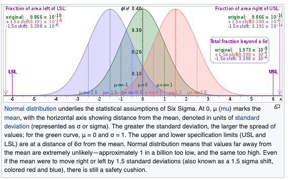
\(6\sigma\) is a widely used tool in TQM [total quality management]. But \(6\sigma\) isn’t actually \(6\sigma\). The famous mantra that goes with it is 3.4 dipmo [defects per million opportunities]. This means that the outer limit [and it only considers one-sided/tailed] on defects is 0.0000034.
The Probability Distribution
How’s that done?
options(scipen=8)library(radiant)result <-prob_norm(mean =0, stdev =1, plb =0.0000034)summary(result, type ="probs")
Probability calculator
Distribution: Normal
Mean        : 0
St. dev     : 1
Lower bound : 0.0000034
Upper bound : 1

P(X < -4.5) = 0.0000034
P(X > -4.5) = 1
\(6\sigma\) is only \(4.5\).
Six Sigma from Wikipedia
How’s that done?
plot(result, type ="probs") +theme_minimal()
Take Away
There are two sources of variation: realizations and averages and both vary. 4.5 \(\sigma\) in the data and \(1.5\sigma\) in the average. Total is six.